Healthy control samples together
Last compiled on 17 November, 2022
Load libraries
library(Seurat)
library(plyr)
library(ggplot2)
library(DropletUtils)
library(celda)
library(SingleCellExperiment)
library(scater)
library(scran)
library(scDblFinder)
library(viridis)
library(MASS)
library(patchwork)
library(harmony)
library(readr)
library(dplyr)
library(clustree)
Load extra functions and sources
get_density <- function(x, y, ...) { # function from https://slowkow.com/notes/ggplot2-color-by-density/
  dens <- MASS::kde2d(x, y, ...)
  ix <- findInterval(x, dens$x)
  iy <- findInterval(y, dens$y)
  ii <- cbind(ix, iy)
  return(dens$z[ii])
}

fancy_scientific <- function(l) { # function from https://stackoverflow.com/a/24241954
     # turn in to character string in scientific notation
     l <- format(l, scientific = TRUE)
     # quote the part before the exponent to keep all the digits
     l <- gsub("^(.*)e", "'\\1'e", l)
     # turn the 'e+' into plotmath format
     l <- gsub("e", "%*%10^", l)
     # return this as an expression
     parse(text=l)
}

setwd("~/000_GitHub/ibd-bcn_single_cell")
source('source/functions_scrnaseq.R')
source('source/colors.R')
Sample Metadata
Metadata of the samples inside the code.
metadata <- data.frame(stringsAsFactors = FALSE, sample = c("SC_002", "SC_004", "SC_005", "SC_008", "SC_010", "SC_011",
    "SC_013", "SC_014", "SC_015", "SC_016", "SC_017", "SC_018", "SC_019", "SC_021", "TOF001W0", "TOF002W0", "TOF005W0",
    "TOF010W0"), sample_name = factor(c("HC 1", "CD 1", "CD 2", "UC 1", "UC 2", "HC 2", "CD 3", "CD 4", "HC 3", "HC 4",
    "HC 5", "HC 6", "CD 5", "CD 6", "UC 3", "UC 4", "UC 5", "UC 6"), levels = c("HC 1", "HC 2", "HC 3", "HC 4", "HC 5",
    "HC 6", "CD 1", "CD 2", "CD 3", "CD 4", "CD 5", "CD 6", "UC 1", "UC 2", "UC 3", "UC 4", "UC 5", "UC 6")), Health = factor(c("HC",
    "CDa", "CDa", "UCa", "UCa", "HC", "CDa", "CDa", "HC", "HC", "HC", "HC", "CDa", "CDa", "UCa", "UCa", "UCa", "UCa"),
    levels = c("HC", "CDa", "UCa")), Health_2 = factor(c("HC", "IBD", "IBD", "IBD", "IBD", "HC", "IBD", "IBD", "HC", "HC",
    "HC", "HC", "IBD", "IBD", "IBD", "IBD", "IBD", "IBD"), levels = c("HC", "IBD")))
Data together (Seurat)
We will only join samples from HC. This code consists of a loop
joining the data. First loads the sample, adds the sample’s metadata
m4, and calculates the doublets and MT%. Puts each sample
in an empty list list_data, and after the loop, merges the
samples of the list using Seurat’s function merge into the
new seudata object.
setwd('~/data_Albas/DATA/') # Dir where we have a folder per sample, with the 3 files from
# outs/filtered_feature_bc_matrix from cellranger output.

list_files <- metadata$sample[metadata$Health == 'HC']
list_data <- list() # empty list

for(i in list_files){
  # read the files
  sce2 <- Read10X(i)

  # feature filtering
  keep_feature <- rowSums(sce2 > 0) > 0
  sce2 <- sce2[keep_feature, ]

  # doublet finding
  sce2 <- scDblFinder(sce2, verbose=FALSE)

  # metadata of sample
  m4 <- data.frame('sample' = rep(i, ncol(sce2)),
                   'doublet' = sce2$scDblFinder.class,
                   'Health' = rep(metadata[metadata$sample == i, 'Health'][1],
                                  ncol(sce2)),
                   'sample_name' = rep(metadata[metadata$sample == i,
                                                'sample_name'][1], ncol(sce2)),
                   'Health_2' = rep(metadata[metadata$sample == i,
                                             'Health_2'][1], ncol(sce2))
  )

  # identify sample per colname
  colnames(sce2) <- paste(i, colnames(sce2), sep='_')
  rownames(m4) <- colnames(sce2)

  # seurat of the sample
  data <- CreateSeuratObject(
    counts(sce2),
    min.features = 100,
    project = i,
    assay = "RNA",
    meta.data = m4
  )

  # calcules the percent.mt per sample
  data[["percent.mt"]] <- PercentageFeatureSet(object = data, pattern = "^MT-")

  # add each sample into the empty list
  list_data[[i]] <- data
}

seudata <- list_data[[1]]
for(i in 2:length(list_files)){
  seudata <- merge(seudata, list_data[[i]])
}
Data exploration
Violin plots
Let’s check the MT% per cell and the number of genes per cell in each sample.
VlnPlot(seudata, features = c('percent.mt', 'nFeature_RNA'),
        group.by = 'sample_name', pt.size = 0) &
  theme(text = element_text(family = 'Helvetica', size = 10),
        axis.text.x = element_text(angle = 90, vjust = 0.5,
                                   family = 'Helvetica', size = 10),
        axis.title.x = element_blank(),
        axis.text.y = element_text(family = 'Helvetica', size = 10)) &
  scale_fill_manual(values = c('#71ad96','#5fb392','#71bda0',
                               '#77c9a9','#82ceb1','#9debcc'))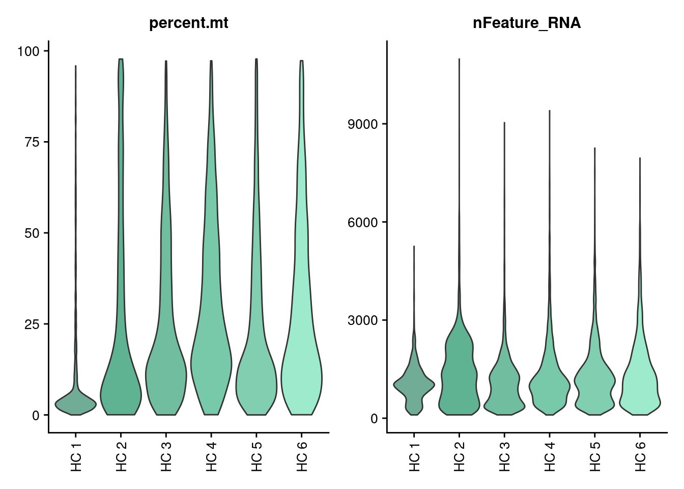
Scatter plot
Let’s check the distribution of the cells considering the total number of counts and the total number of genes per cell. First plot is colored by doublet. Second plot is colored by sample_name.
meta <- seudata@meta.data
meta <- meta[order(meta$doublet, decreasing = T),]
ggplot(meta) +
  geom_point(aes(nCount_RNA, nFeature_RNA, color = doublet), size=0.2) +
  theme_classic() +
  scale_color_manual(values = c('doublet' = '#F6AE2DCC',
                                'singlet' = '#86BBD860'))+
  theme(plot.title = element_text(size = 25))+
  scale_x_continuous(labels=fancy_scientific) +
  scale_y_continuous(labels=fancy_scientific) +
  theme(text = element_text(family = 'Helvetica', size = 10),
        axis.text.x = element_text(family = 'Helvetica', size = 10),
        axis.text.y = element_text(family = 'Helvetica', size = 10),
        legend.key.size = unit(5,"bigpts"), legend.title = element_blank())+
  guides(color = guide_legend(override.aes = list(size = 1.2)))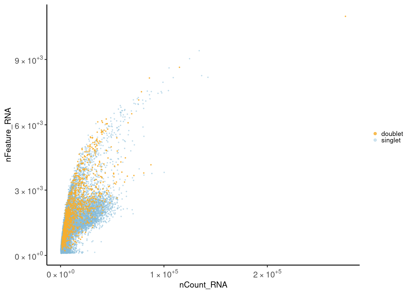
Data filtering
We first filter out the cells that are considered doublets and let’s recheck the distribution of the cells after filtering.
Pre-filtering cells/sample
Tables showing the number of cells classified as singlet and doublet.
The table shows the global numbers. The barplot shows singlets/doublets
per sample. In the code, we filter out the cells classified as doublet
into a new object seudataf.
ta <-  as.data.frame(table(seudata$doublet))
colnames(ta) <- c('category', 'n_cells')
knitr::kable(ta)| category | n_cells |
|---|---|
| doublet | 1125 |
| singlet | 18519 |
ta2 <- as.data.frame(table(seudata$sample_name, seudata$doublet))
colnames(ta2) <- c('sample','doublet','n_cells')
ta2$sample <- factor(ta2$sample,
                     levels = c("HC 1", "HC 2", "HC 3", "HC 4","HC 5", "HC 6"))
ggplot(data=ta2, aes(x=sample, y=n_cells, fill=doublet)) +
  geom_bar(stat="identity", position=position_dodge())+
  geom_text(aes(label=n_cells), vjust=1.6, color="black",
            position = position_dodge(0.9), size=2.5)+
  scale_fill_manual(values = c('doublet' = '#F6AE2DCC',
                               'singlet' = '#86BBD860'))+
  labs(y = 'number of cells') +
  theme_classic()+
  theme(axis.text.x = element_text(angle=90, vjust=0.5),
        legend.title = element_blank(),
        axis.title.x= element_blank())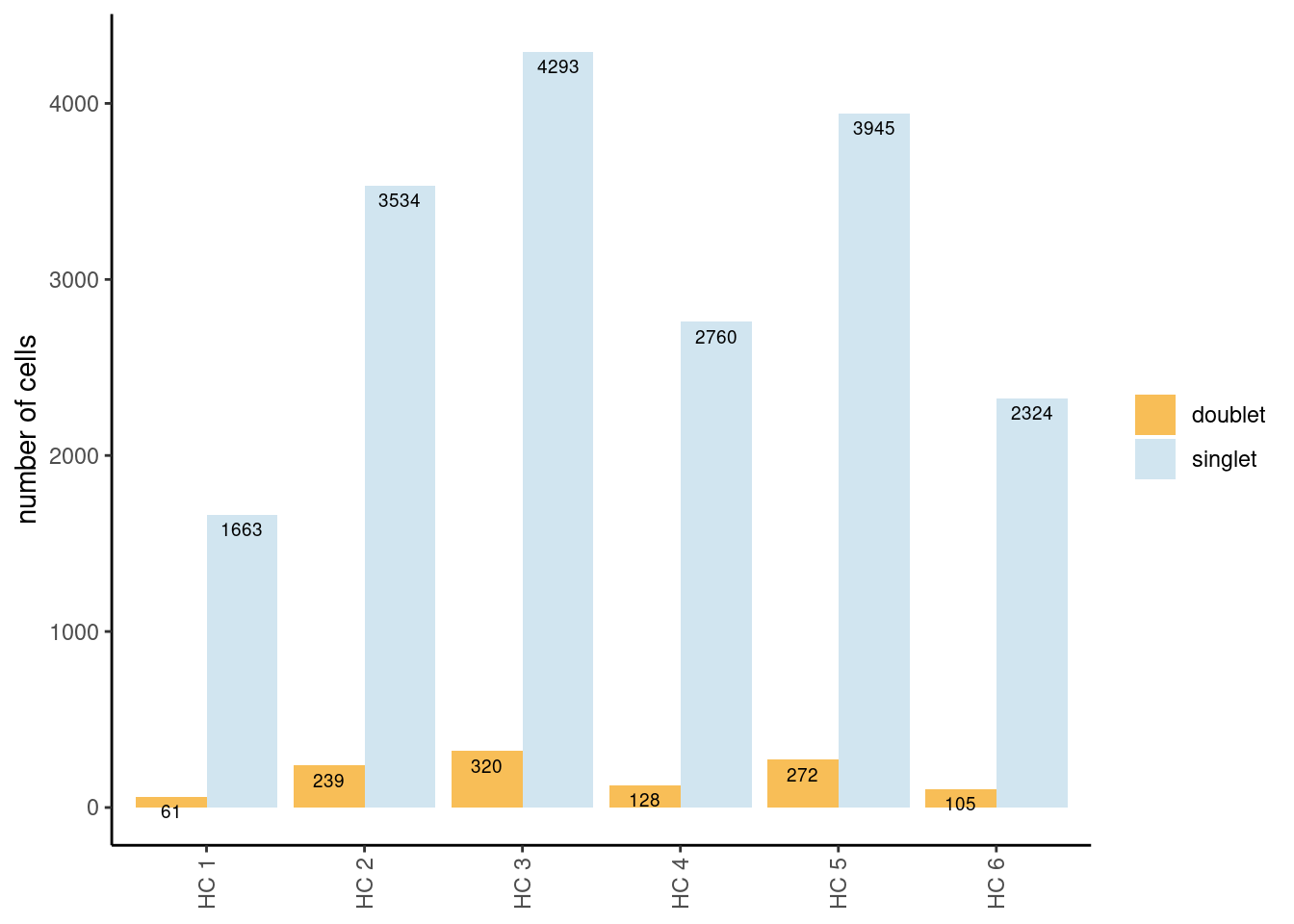
Distribution after doublet filtering
Distribution of cells in the scatter plot (ncount/nfeatures) without the doublets.
seudataf <- seudata[,seudata$doublet == 'singlet']

meta_dot <-  seudataf@meta.data[sample(1:nrow(seudataf@meta.data)), ]
ggplot(meta_dot) +
  geom_point(aes(x = nCount_RNA, y = nFeature_RNA, color = sample_name),
             size = 0.2) +
  theme_classic()+
  scale_x_continuous(labels=fancy_scientific) +
  scale_y_continuous(labels=fancy_scientific) +
  scale_color_brewer(palette = 'Set1')+
  guides(color = guide_legend(override.aes = list(size = 1.2), ncol=1))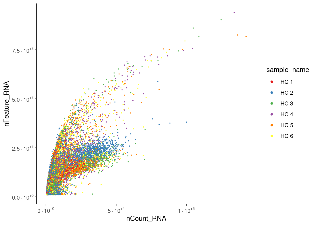
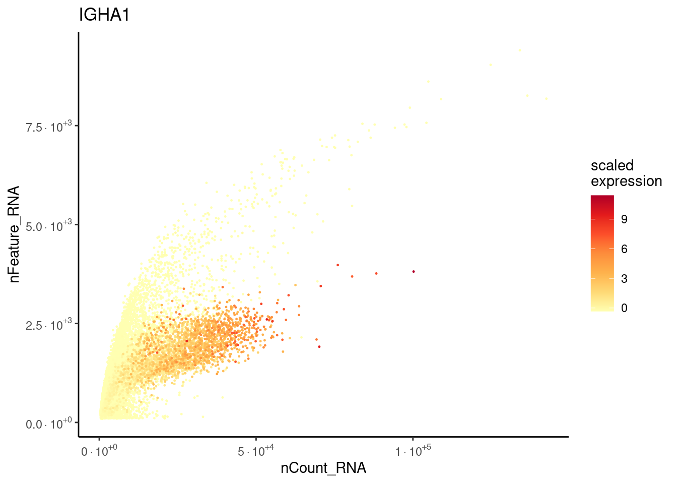
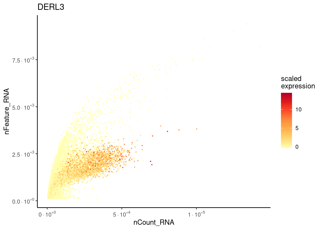
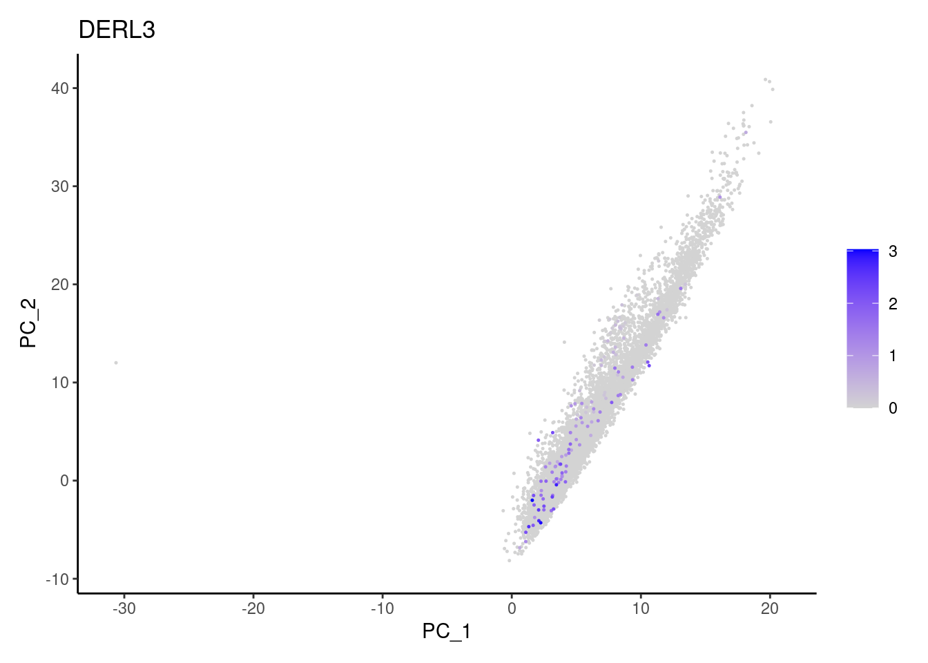
Plasmacells have more counts/genes than other cell types.
plasma_genes <- c('IGHA1', 'DERL3')
meta_dot <-  FetchData(seudataf, vars = c('nCount_RNA', 'nFeature_RNA',plasma_genes))

for (gene in plasma_genes) {
  meta_dot$expression <- scale(meta_dot[, gene] )
  meta_dot <- meta_dot[order(meta_dot$expression), ]

  p <- ggplot(meta_dot) +
  geom_point(aes(x = nCount_RNA, y = nFeature_RNA, color = expression),
             size = 0.2) +
  scale_color_distiller("scaled\nexpression",
                        limits = c(min(meta_dot$expression, na.rm = T),
                                   max(meta_dot$expression, na.rm=T)),
                        na.value = "white", palette = "YlOrRd", direction = 1) +

  theme_classic() + labs(title = gene) +
  scale_x_continuous(labels=fancy_scientific) +
  scale_y_continuous(labels=fancy_scientific)

  cat("### ", gene, "\n"); print(p); cat("\n\n")

}
IGHA1
DERL3
MT% filtering after doublet filtering
Distribution of cells in scatter plot (nfeatures/percent.mt) to check where are the majority of our cells. We can see the dots colored by density using the function get_density shown in Load extra functions and sources. Most cells are located between 0 and 25% MT. Nevertheless, let’s check the higher % of MT in more detail.
Density plot
meta <- seudataf@meta.data
meta$density <- get_density(meta$percent.mt, meta$nFeature_RNA, n = 100)
ggplot(meta) +
  geom_point(aes(percent.mt, nFeature_RNA, color = density), size = 0.2) +
  scale_color_viridis() + theme_classic() +
  theme(text = element_text( size = 12),
        axis.title = element_text( size = 12),
        legend.text = element_blank())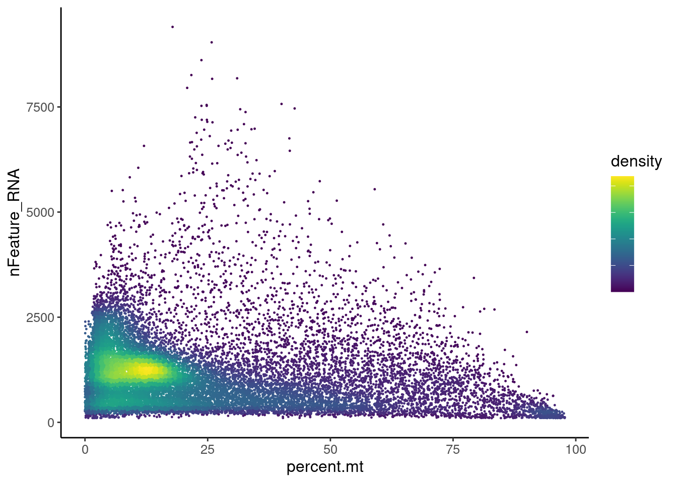
Density plot > 25%
meta2 <- seudata@meta.data[seudata@meta.data$percent.mt > 25,]
meta2$density <- get_density(meta2$percent.mt, meta2$nFeature_RNA, n = 100)

ggplot(meta2) +
  geom_vline(xintercept = 65, color = '#7A7A7A', linetype="dashed") +
  geom_vline(xintercept = 95, color = '#7A7A7A', linetype="dashed") +
  geom_point(aes(percent.mt, nFeature_RNA, color = density), size = 0.2) +
  scale_color_viridis() + theme_classic() +
  theme(plot.title = element_text(size = 25))+
  theme(text = element_text( size = 12),
        axis.text.x = element_text( size = 10),
        axis.text.y = element_text( size = 10),
        legend.text = element_blank())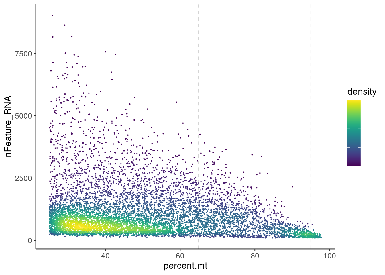
There are two main densities in the plot, one between 25 and 65, and the second around 95%.We keep all cells <65%MT and get rid of the density around 95%, which will bring no information to the data set.
Genes without expression filtering
counts <- seudataf@assays$RNA@counts
pp <- which(Matrix::rowSums(counts)==0)
xx <-setdiff(rownames(seudataf), names(pp))
seudataf <- subset(seudataf, features = xx)
Post-filtering cells/sample
seudataf <- seudataf[, seudataf$percent.mt < 65 & seudataf$nFeature_RNA > 100]

ta3 <- as.data.frame(table(seudataf$sample_name, seudataf$Health))
colnames(ta3) <- c('sample','Health','n_cells')
ta3 <- ta3[ta3$n_cells != 0,]
ta3$sample <- factor(ta3$sample,
                     levels = c("HC 1", "HC 2", "HC 3", "HC 4", "HC 5", "HC 6"))
ta3[,c('sample', 'n_cells')]
##   sample n_cells
## 1   HC 1    1614
## 2   HC 2    3032
## 3   HC 3    3964
## 4   HC 4    2521
## 5   HC 5    3671
## 6   HC 6    2105
ggplot(data=ta3, aes(x=sample, y=n_cells, fill=Health)) +
  geom_bar(stat="identity", position=position_dodge())+
  geom_text(aes(label=n_cells), vjust=1.6, color="black",
            position = position_dodge(0.9), size=2.5)+
  scale_fill_manual(values = colors_health_alpha)+
  labs(y = 'number of cells after MT filter') +
  theme_classic()+
  theme(axis.text.x = element_text(angle=90, vjust=0.5),
        legend.title = element_blank(),
        axis.title.x= element_blank())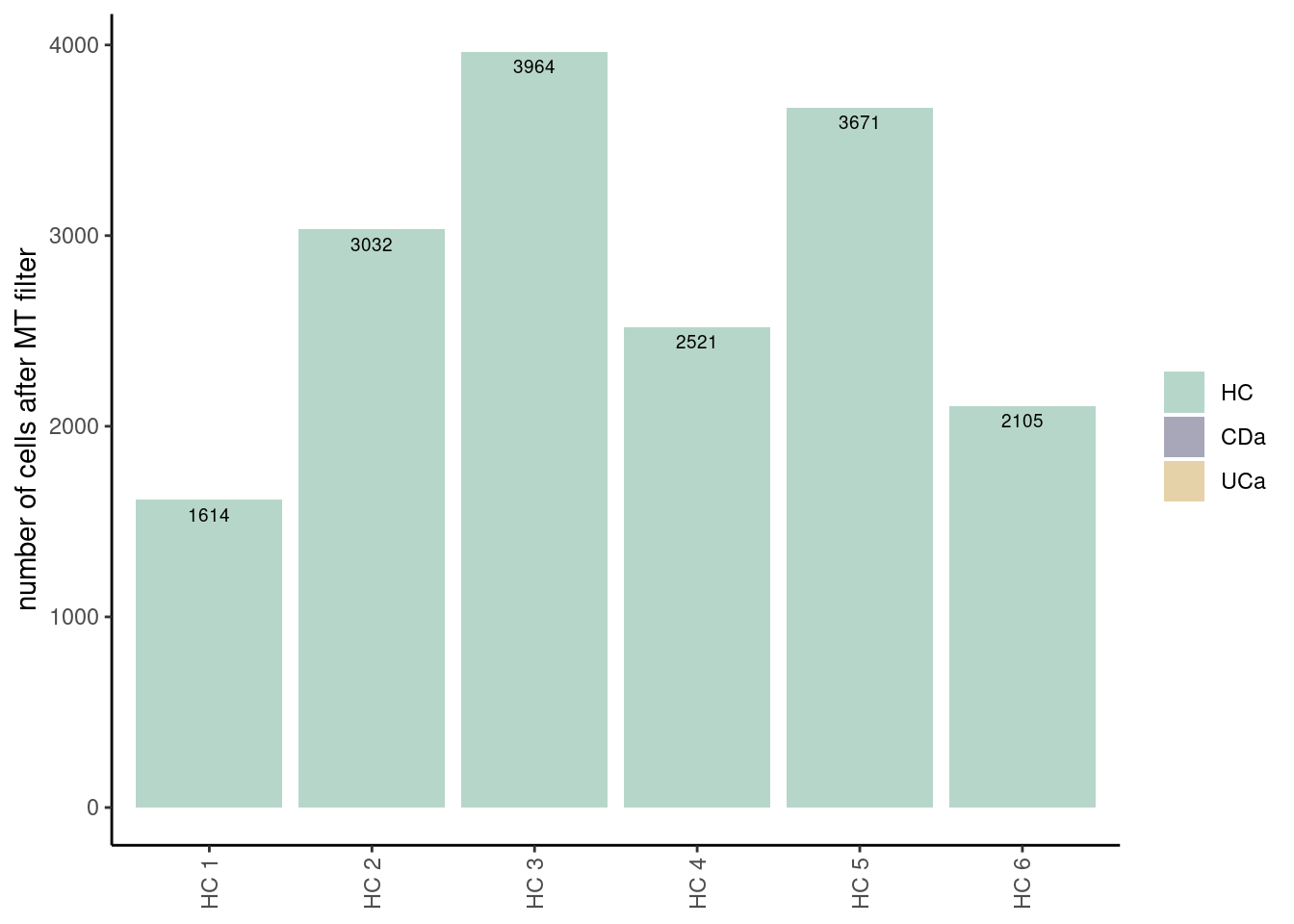
Dimension reduction
PCA calculation
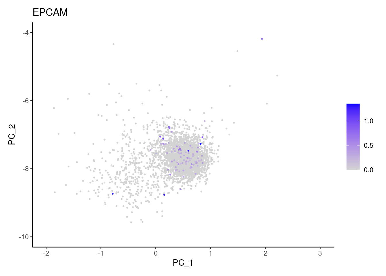
We follow the Seurat protocol. Plot shows the gene expression of CD3E (Tcells), EPCAM (epithelium), DERL3 (plasma cells) and COL3A1 (stromal cells) in the resulting PCA.
seudataf <- seurat_to_pca(seudataf)
## [1] "NORMALIZATION"
## [1] "VARIABLE FEATURES"
## [1] "SCALE DATA"
## Centering and scaling data matrix
## [1] "RUN PCA"
## PC_ 1
## Positive:  LGALS4, KRT8, PIGR, FXYD3, CLDN7
## Negative:  COL1A2, C1S, COL3A1, DCN, A2M
FeaturePlot(seudataf, features = c('CD3E','EPCAM', 'DERL3', 'COL3A1'), order=T) & theme_classic() 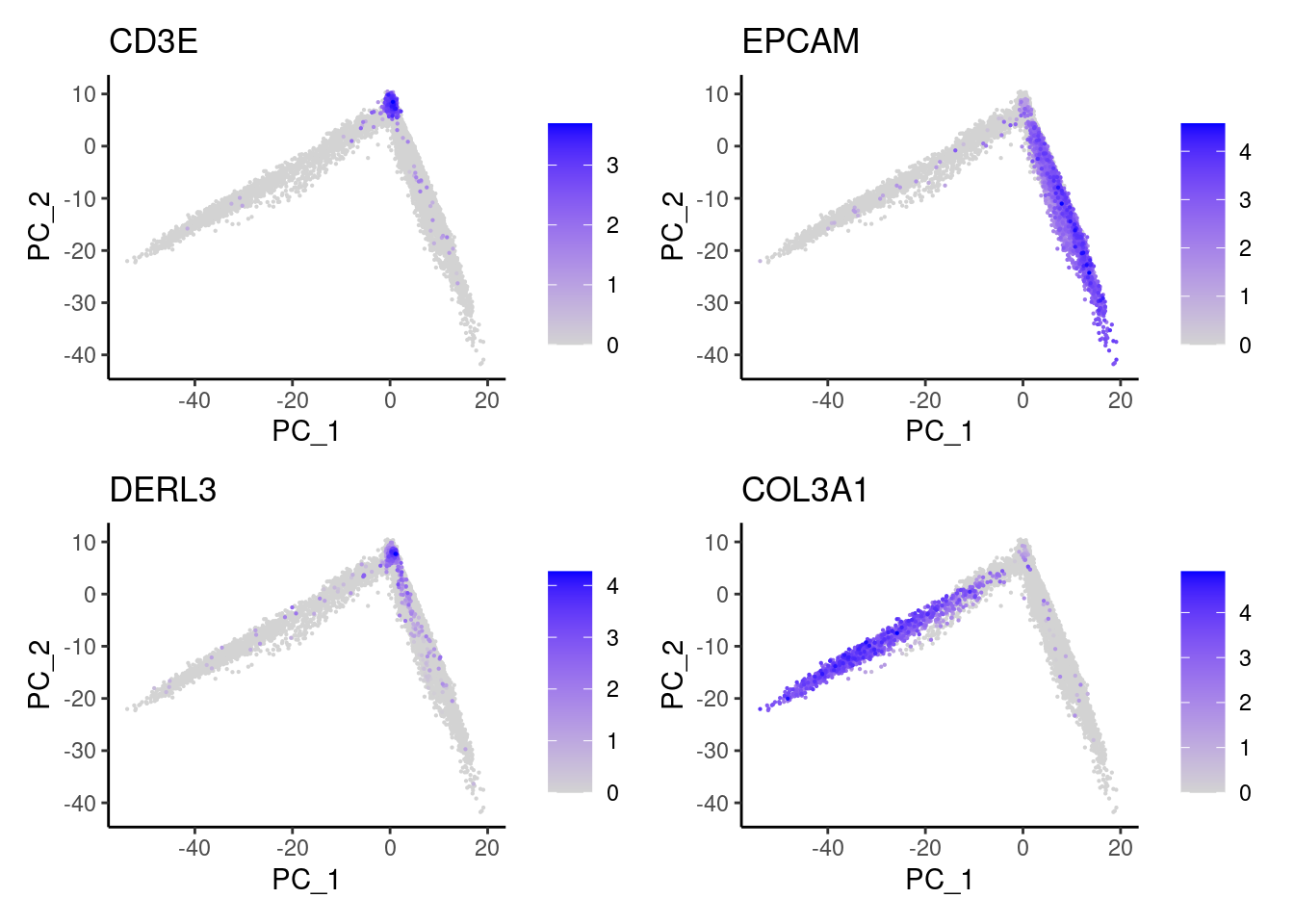
UMAP calculation
We selected 22 PCs from the elbowplot, and generated the UMAP for the HC samples.
a <- ElbowPlot(seudataf, ndims = 100) +
  geom_vline(xintercept = 22, linetype = 2)

seudataf <- FindNeighbors(seudataf, dims = 1:22, reduction = 'pca')
seudataf <- RunUMAP(seudataf, dims=1:22, reduction = 'pca')
b <- DimPlot(seudataf, group.by = 'sample_name') + theme_classic()
a + b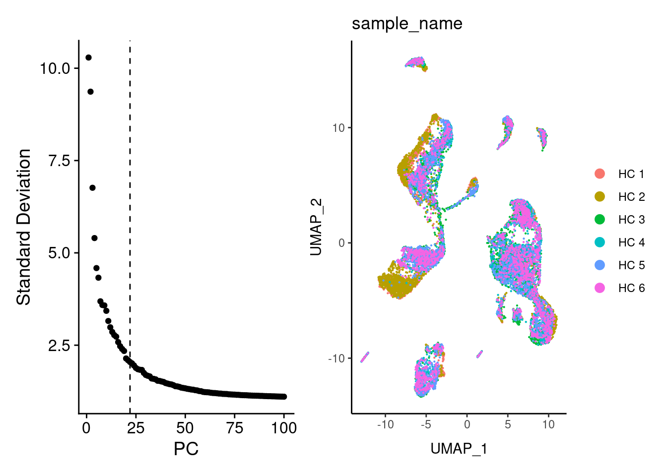
Batch correction
We appreciated a bias for samples HC1 and HC2. We correct by Harmony.
seudataf <- RunHarmony(seudataf, group.by = 'sample_name', dims.use = 1:22)
a <- ElbowPlot(seudataf, ndims = 100, reduction = 'harmony') +
  geom_vline(xintercept = 24, linetype = 2) +
  labs(title = paste0('Harmony - 22PCS'))
seudataf<- FindNeighbors(seudataf, reduction = "harmony", dims = 1:24)
seudataf<-RunUMAP(seudataf, dims=1:24, reduction= "harmony")
b <- DimPlot(seudataf, group.by = 'sample_name') + labs(title='') + theme_classic()

a+b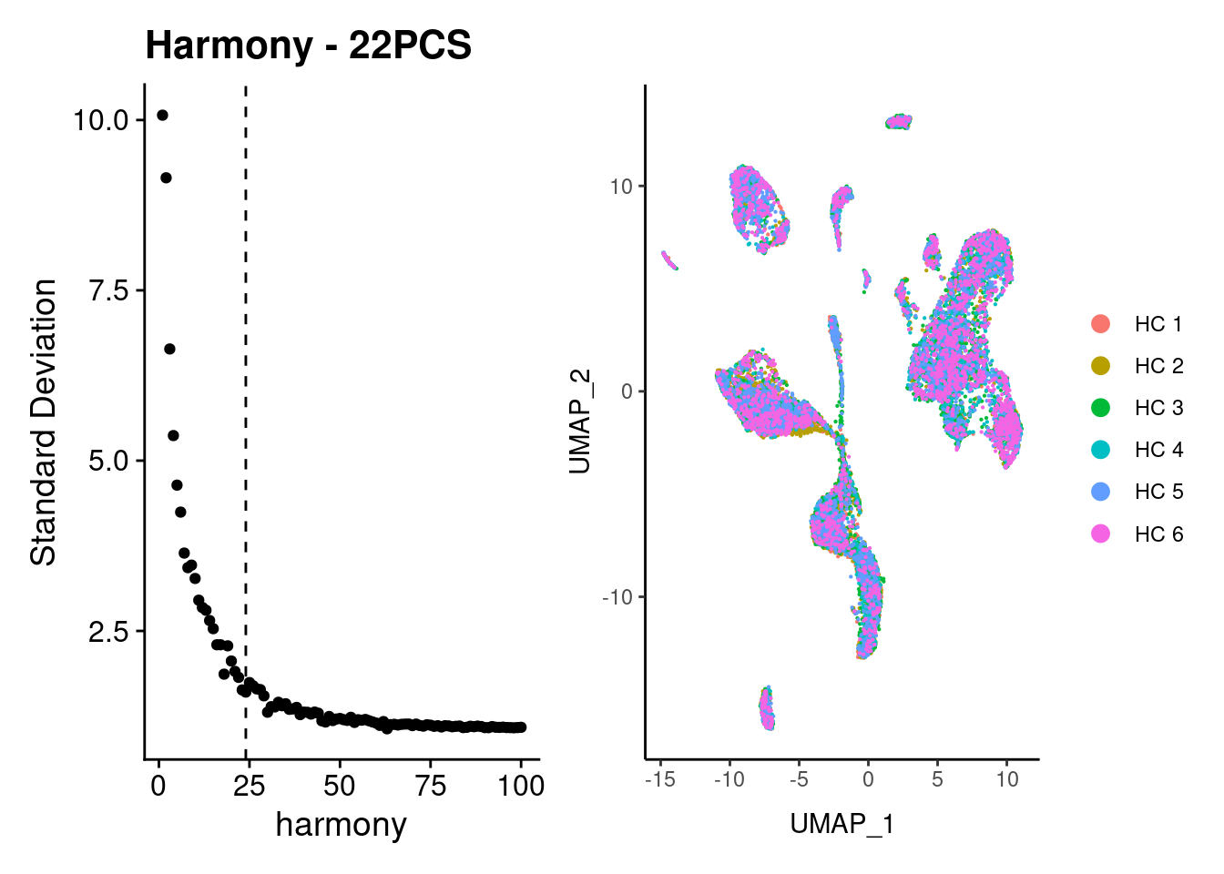
Split the object in 5 major subsets
We cluster the samples using Louvain classification and look for the markers.
dir.create('HC')
dir.create('HC/filter_65')
seudataf <- resolutions(seudataf, resolutions = c(0.1, 0.3, 0.5),
                         workingdir = 'HC/filter_65/',
                         title = 'HC')
saveRDS(seudataf,'HC/filter_65/HC.RDS')
Plot with the three resolutions we tried
a <- DimPlot(seudataf, group.by = 'RNA_snn_res.0.1', label = T)  + theme_classic() + NoLegend()
b <- DimPlot(seudataf, group.by = 'RNA_snn_res.0.3', label = T)  + theme_classic() + NoLegend()
c <- DimPlot(seudataf, group.by = 'RNA_snn_res.0.5', label = T)  + theme_classic() + NoLegend()

(a + b) / (c +  plot_spacer() )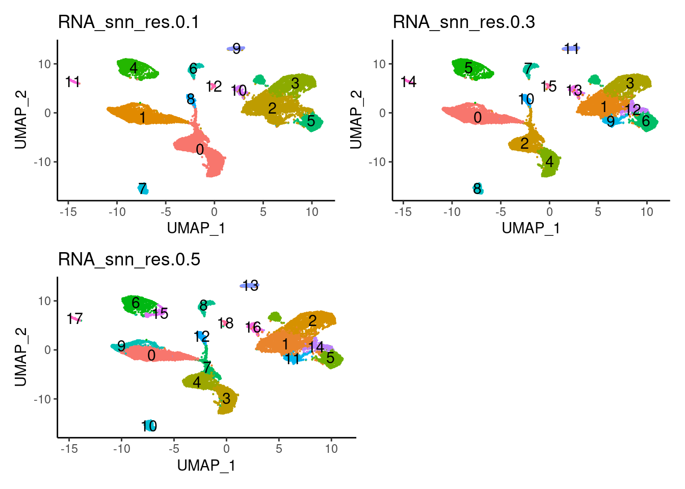
Plot showing the top5 markers
marker_genes <- read_delim("HC/filter_65/HC_markers_resolution_0.1.csv",
                           delim = ";", escape_double = FALSE,
                           locale = locale(decimal_mark = ",", grouping_mark = "."),
                           trim_ws = TRUE)

top5 <- marker_genes %>%
  dplyr::group_by(cluster)%>%
  dplyr::slice(1:5)
top5_g <- unique(top5$gene)

DotPlot(seudataf, features = top5_g, group.by = 'RNA_snn_res.0.1' ) + theme_classic() + theme(axis.text.x = element_text(angle=90), axis.title = element_blank()) + NoLegend() + labs(title = 'Resolution 0.1')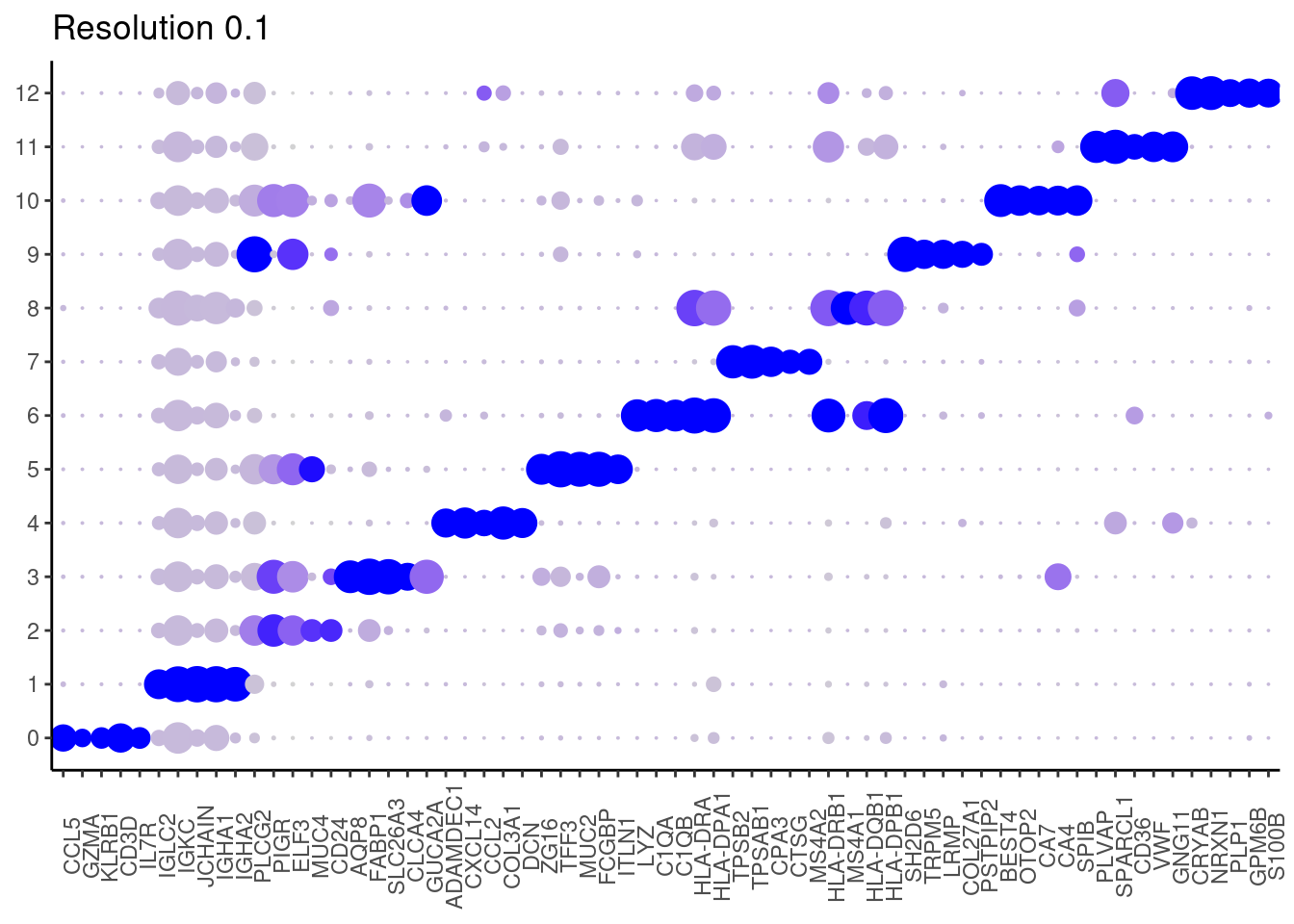
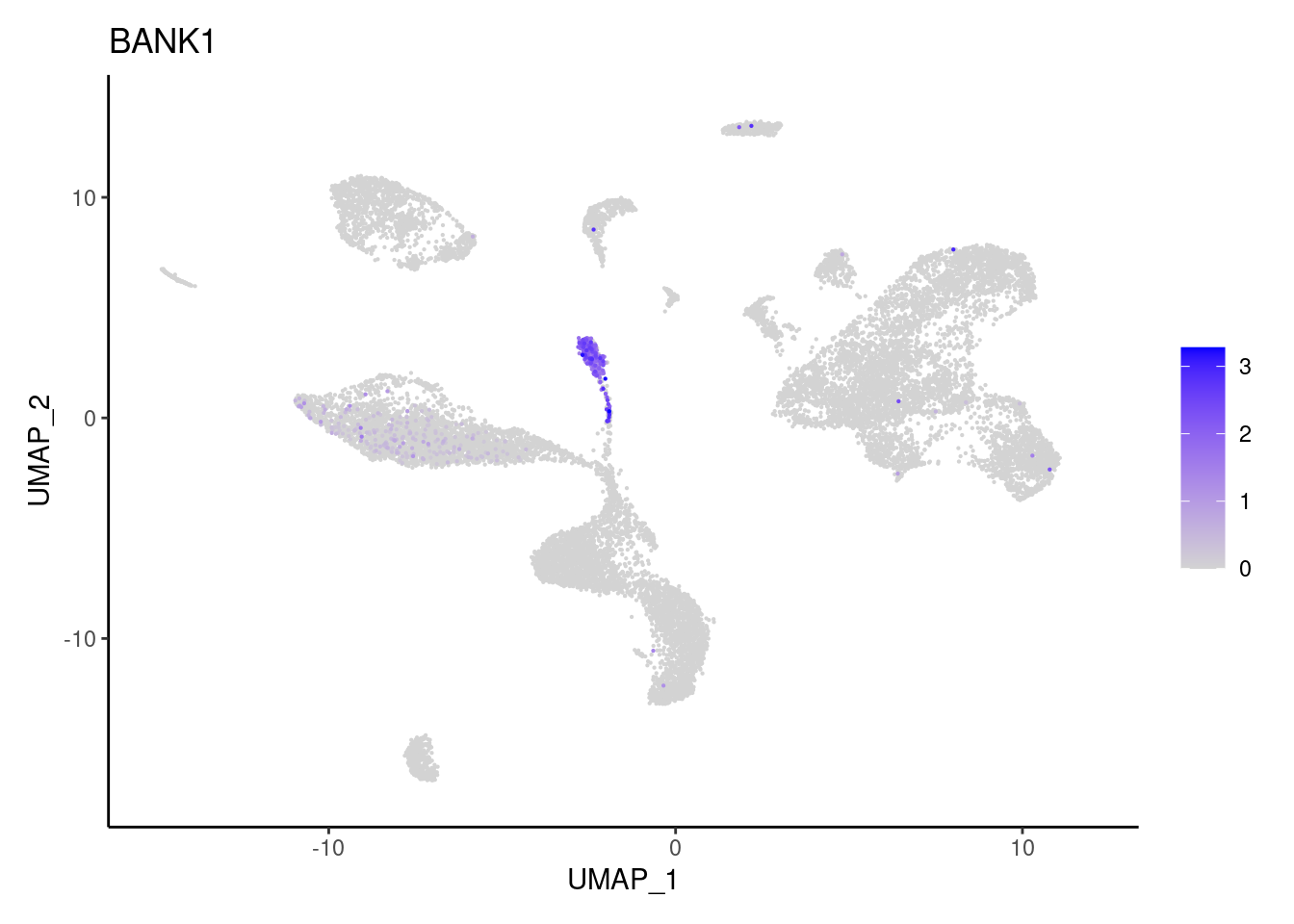
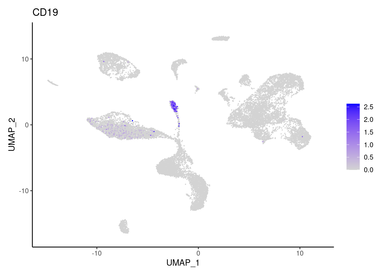
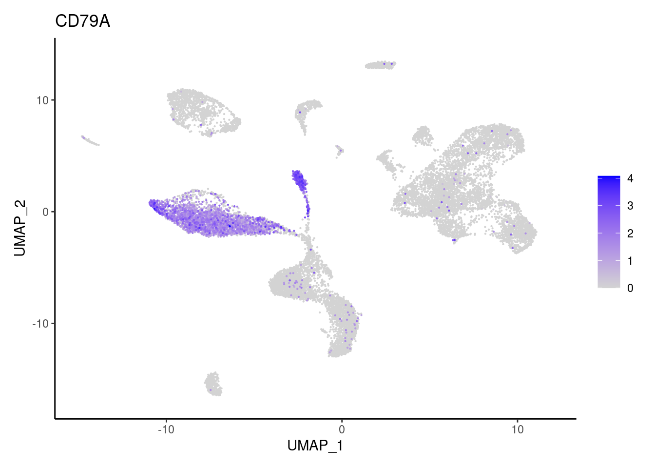
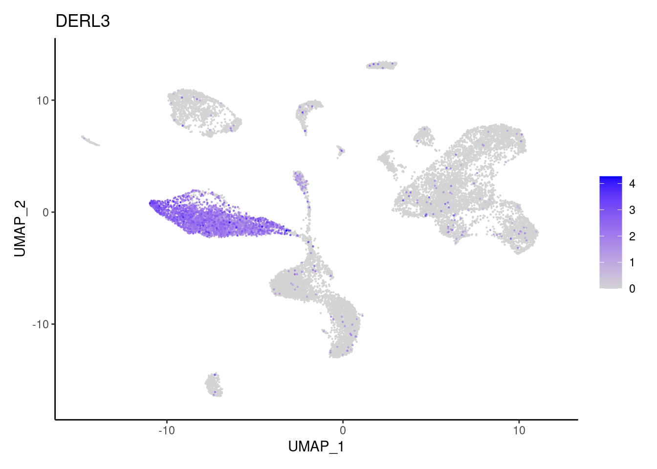
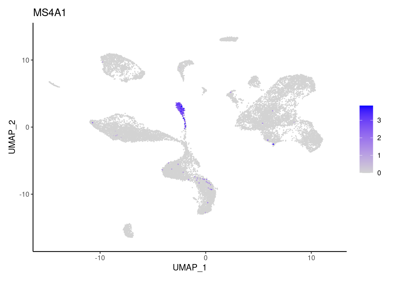
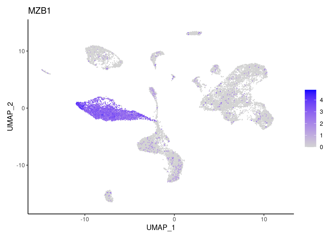
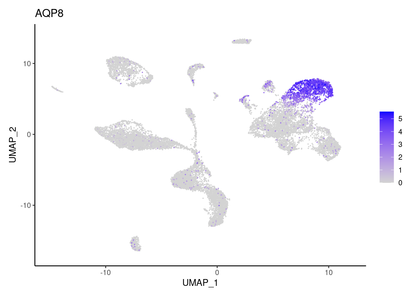
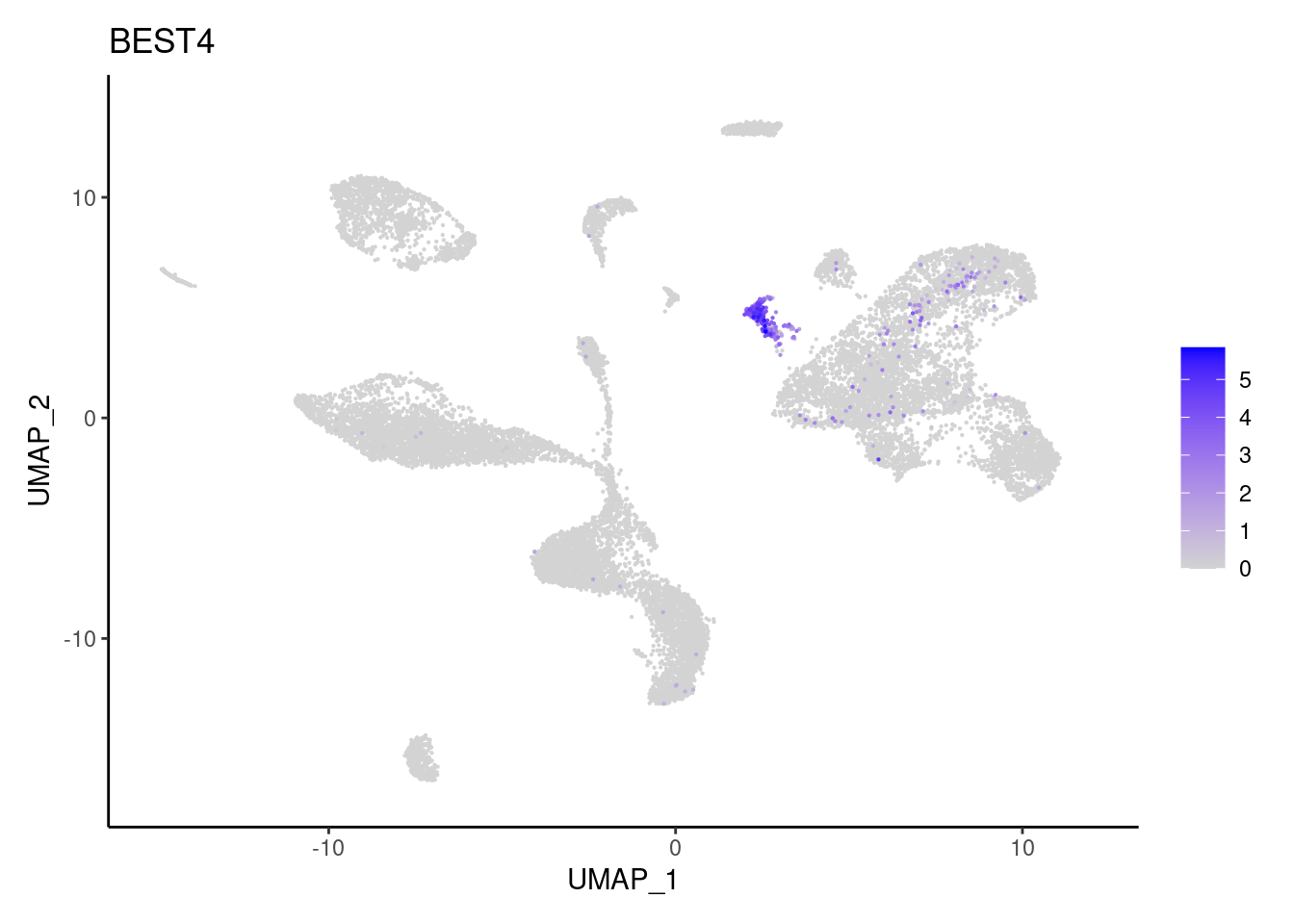
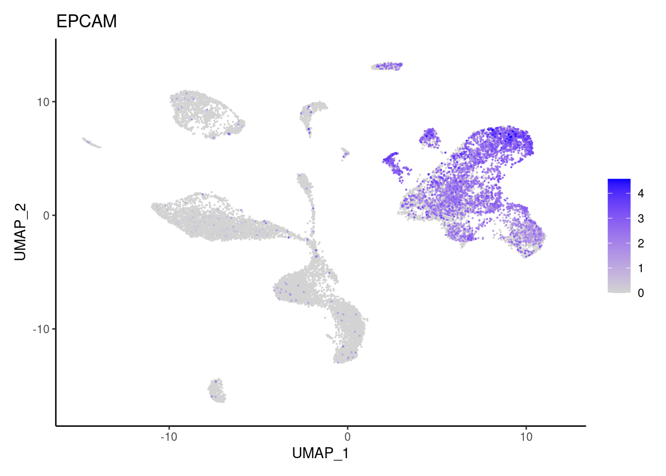
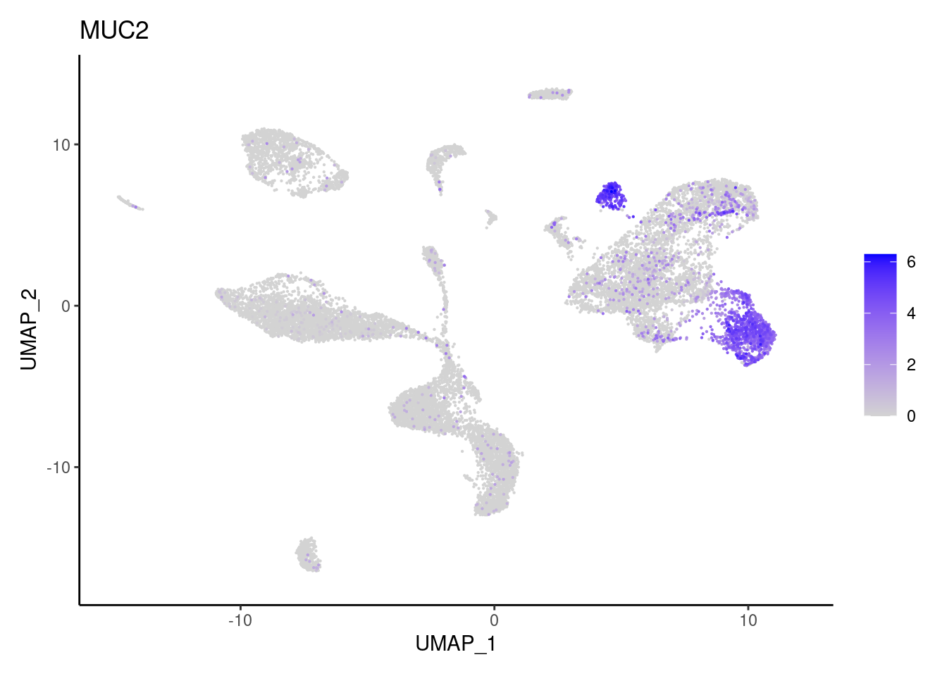
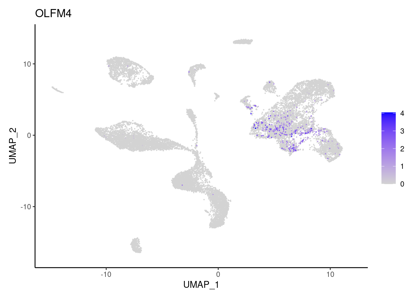
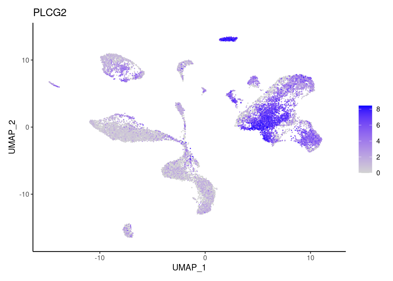
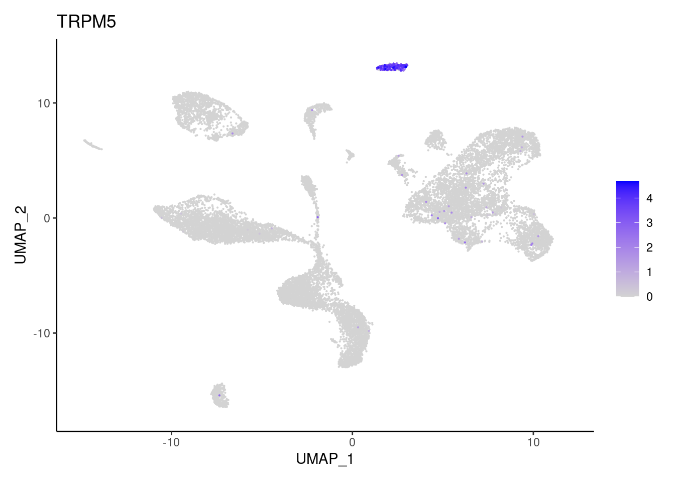
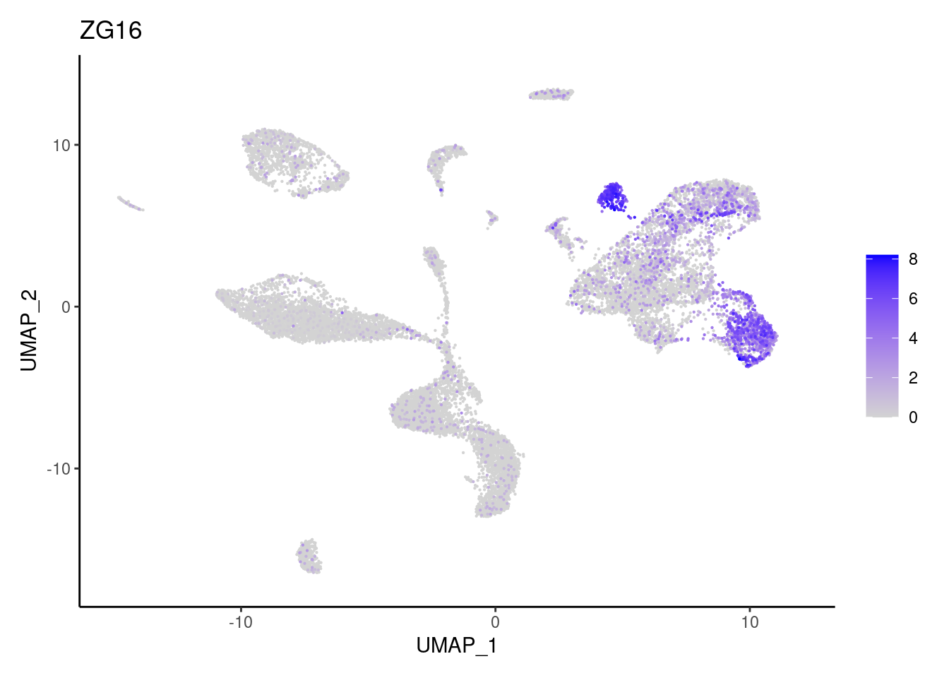
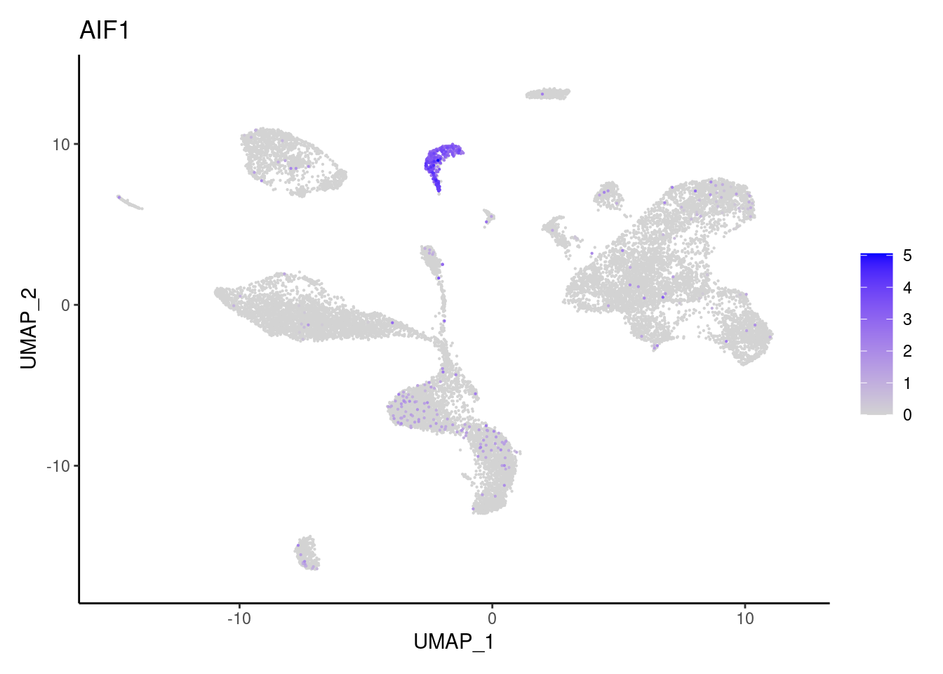
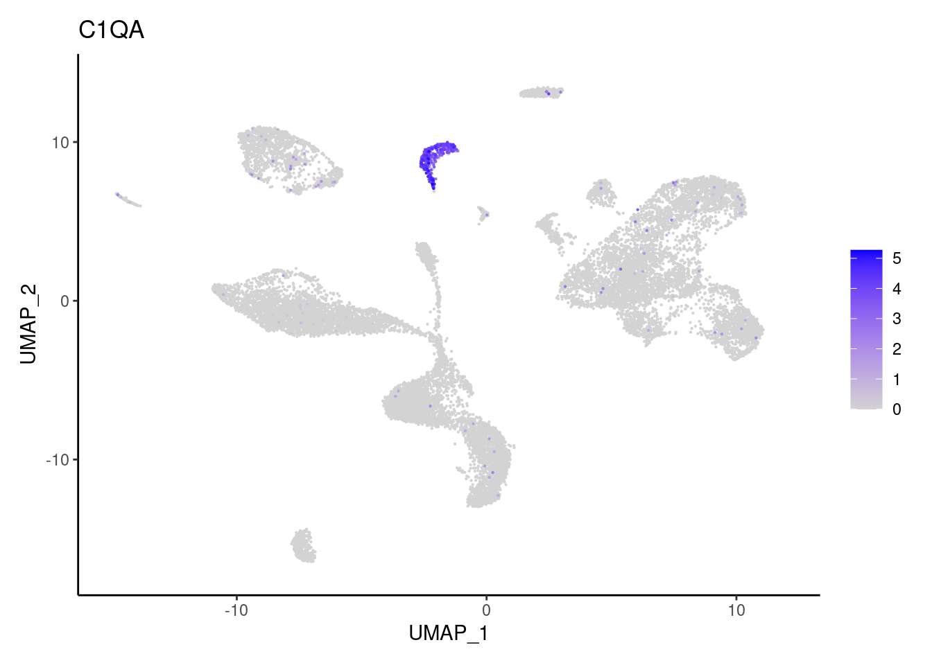
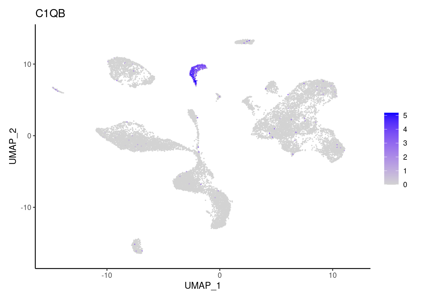
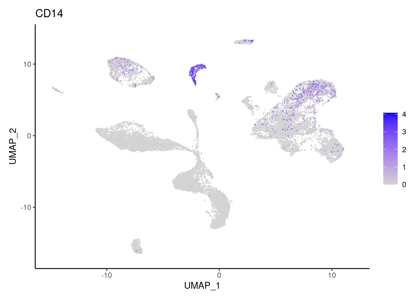
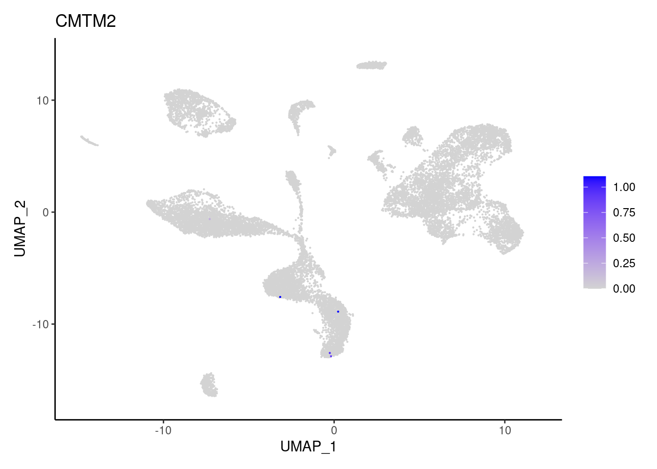
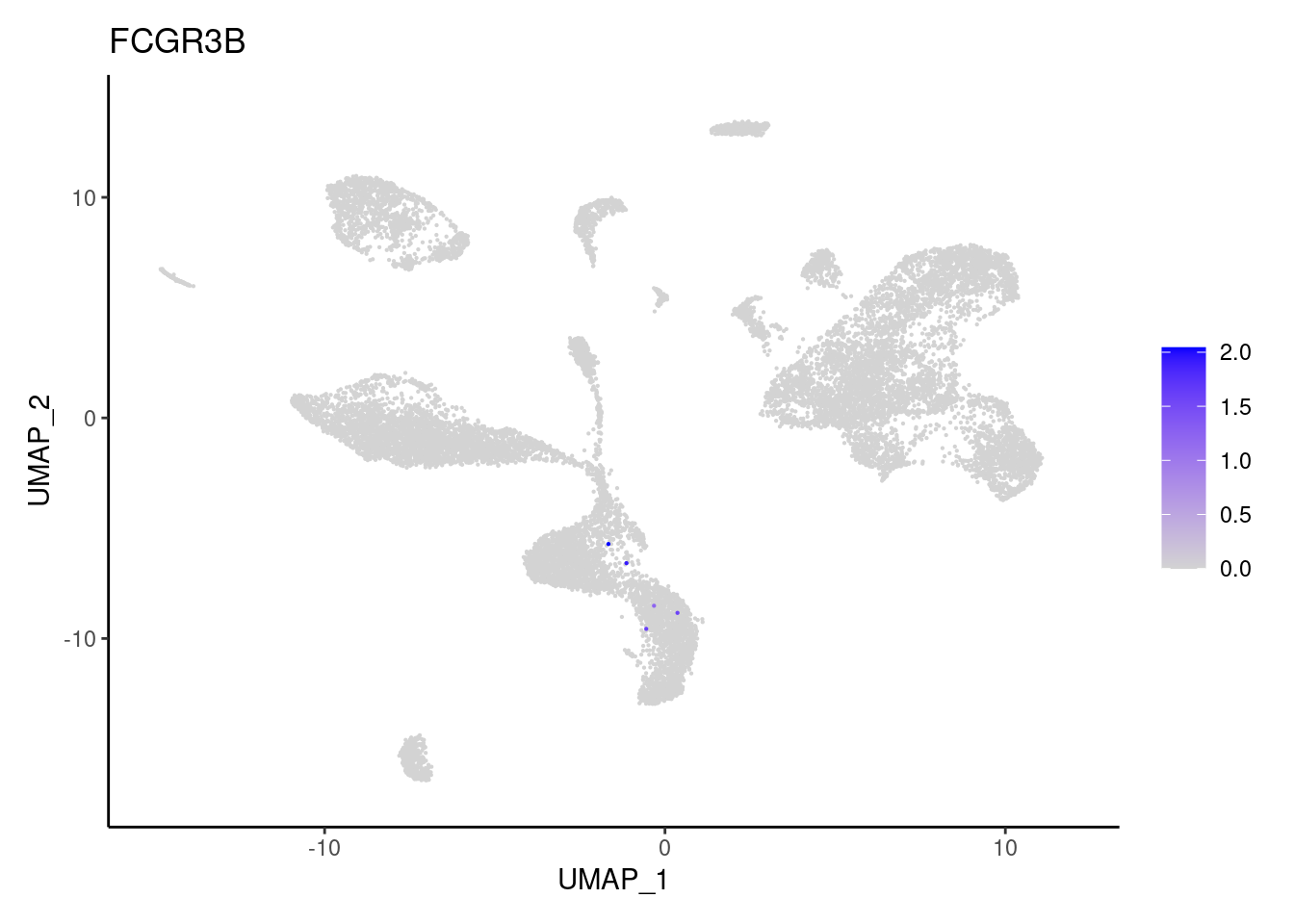
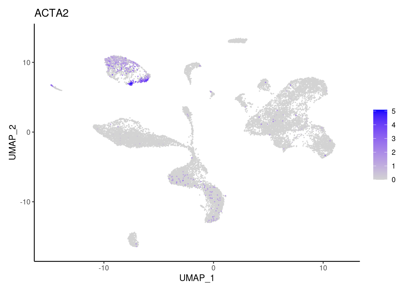
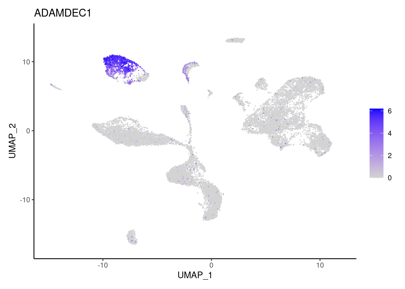
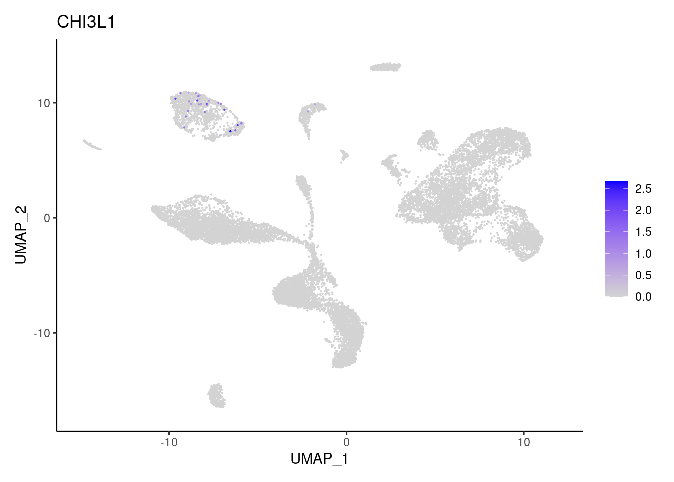
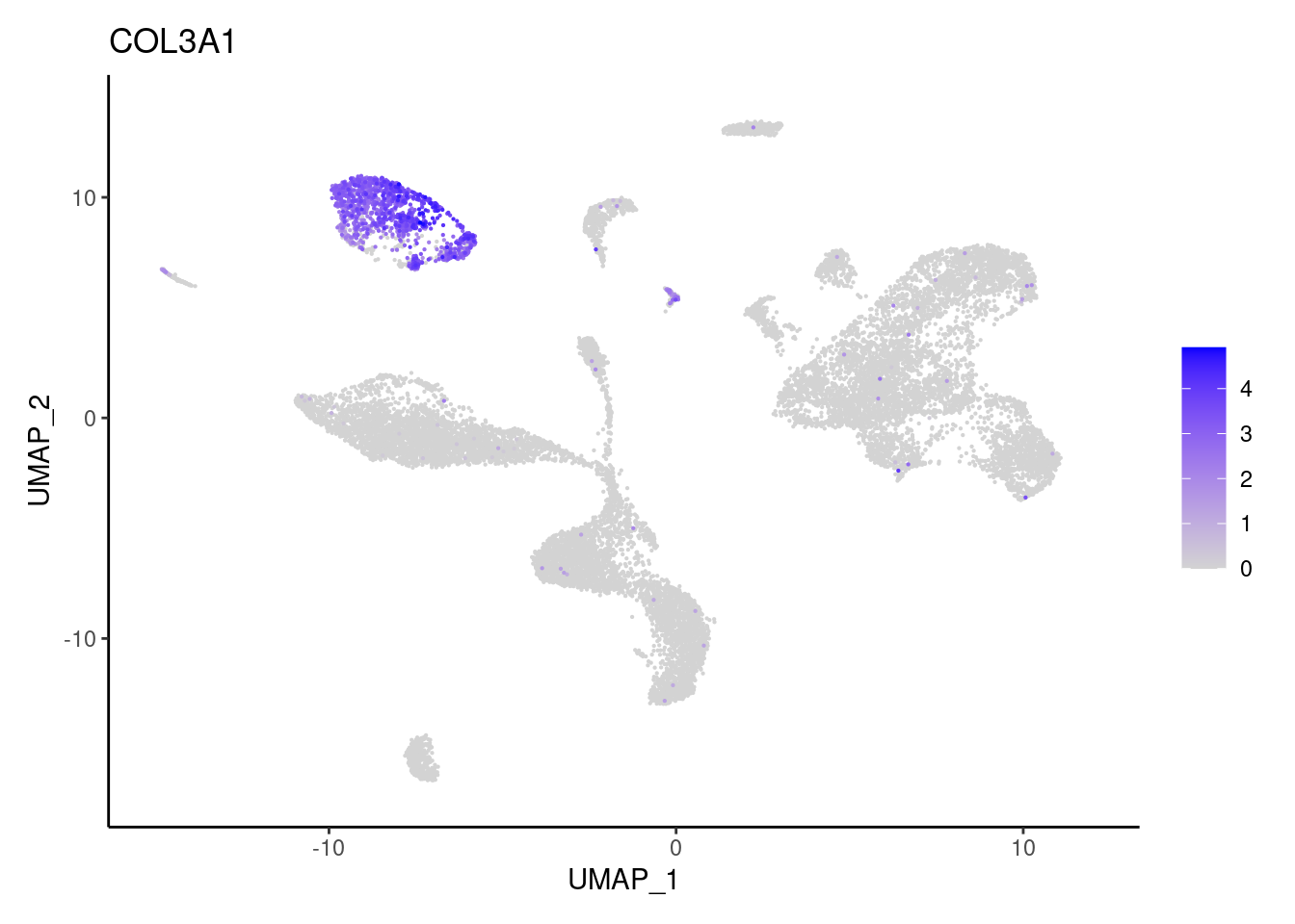
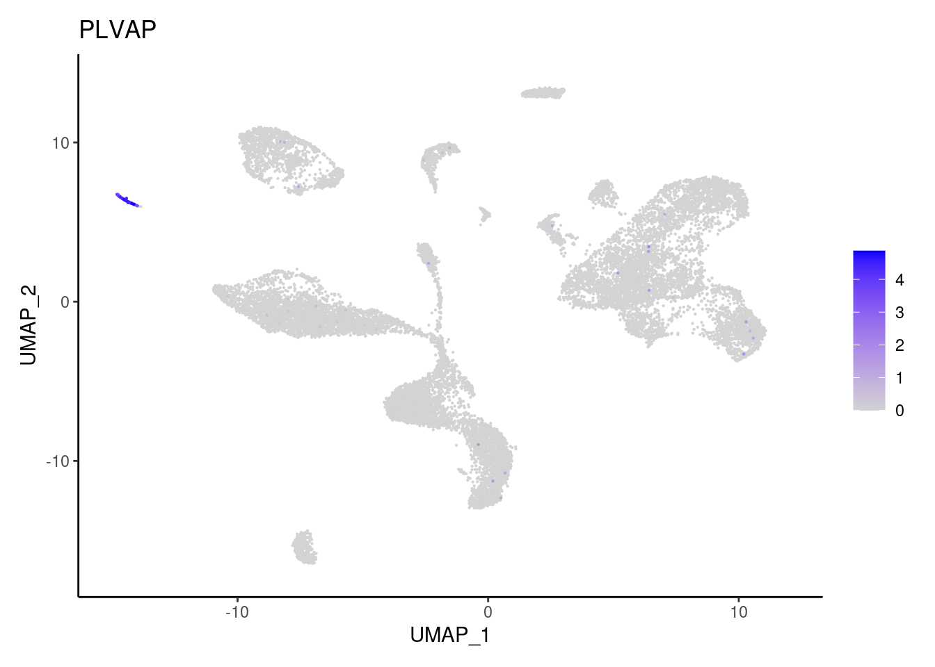
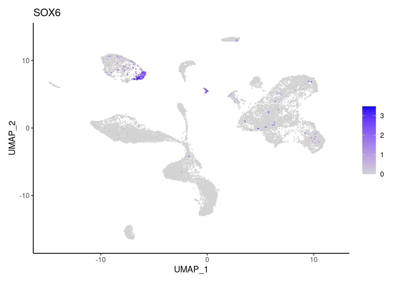
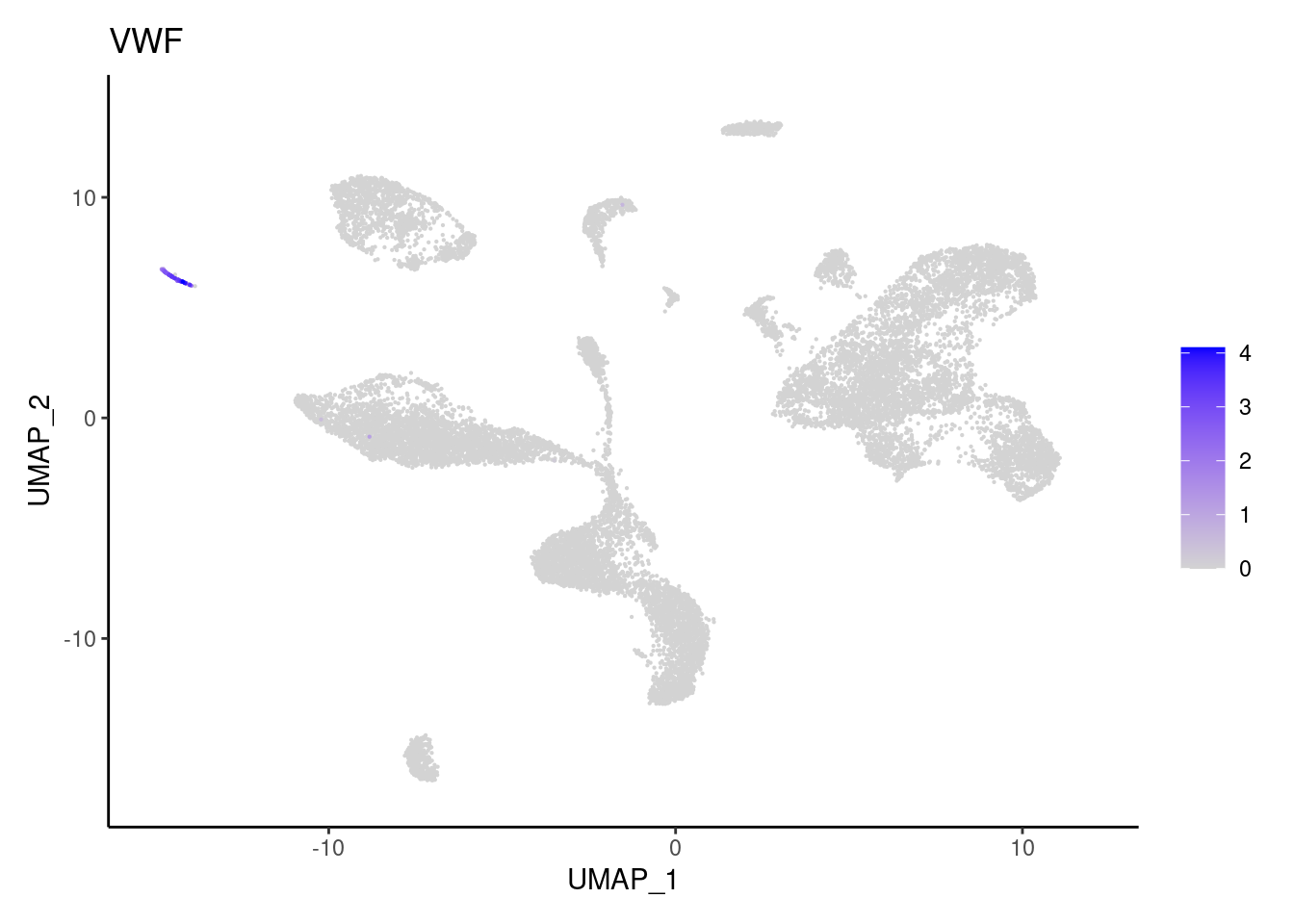
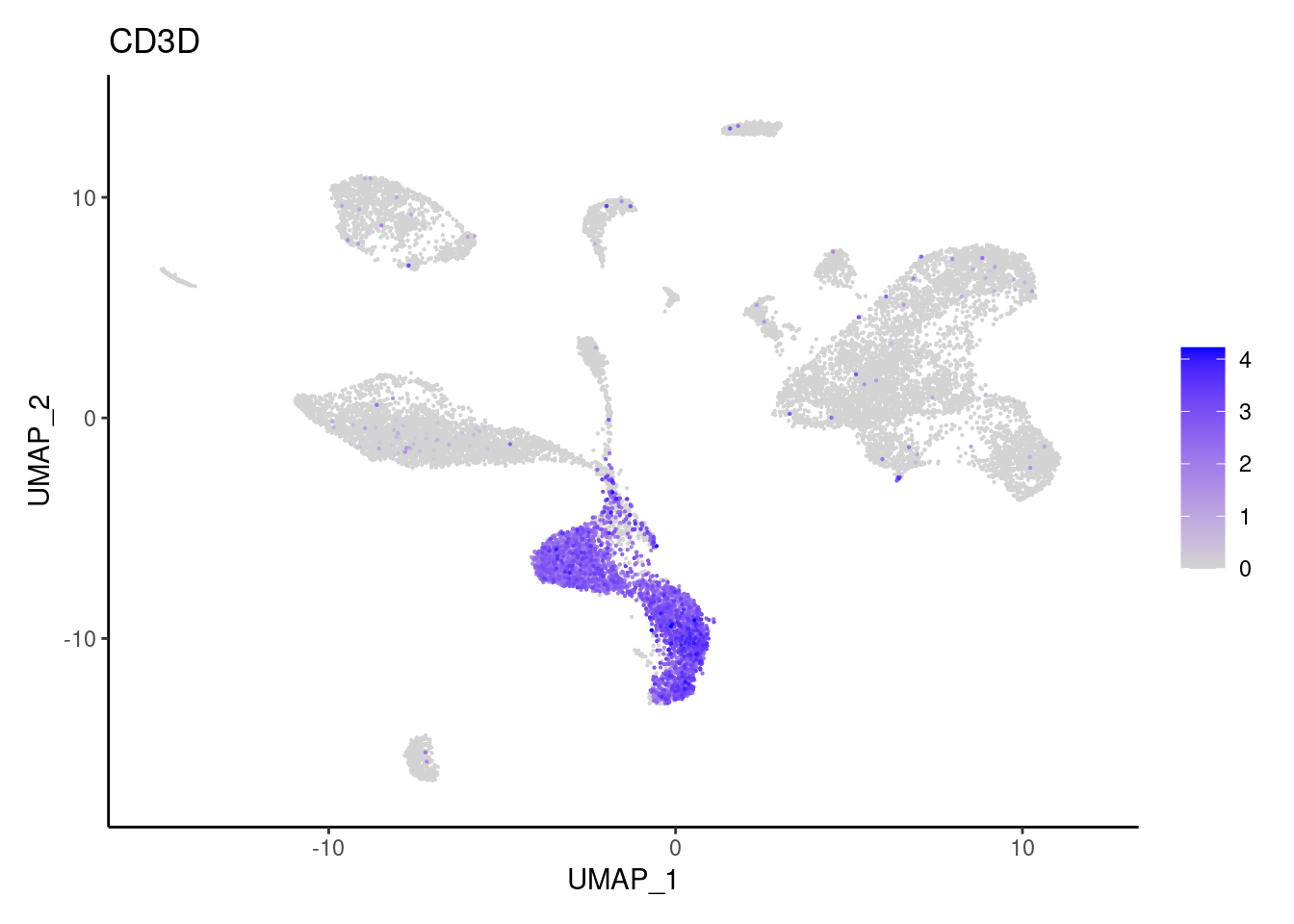
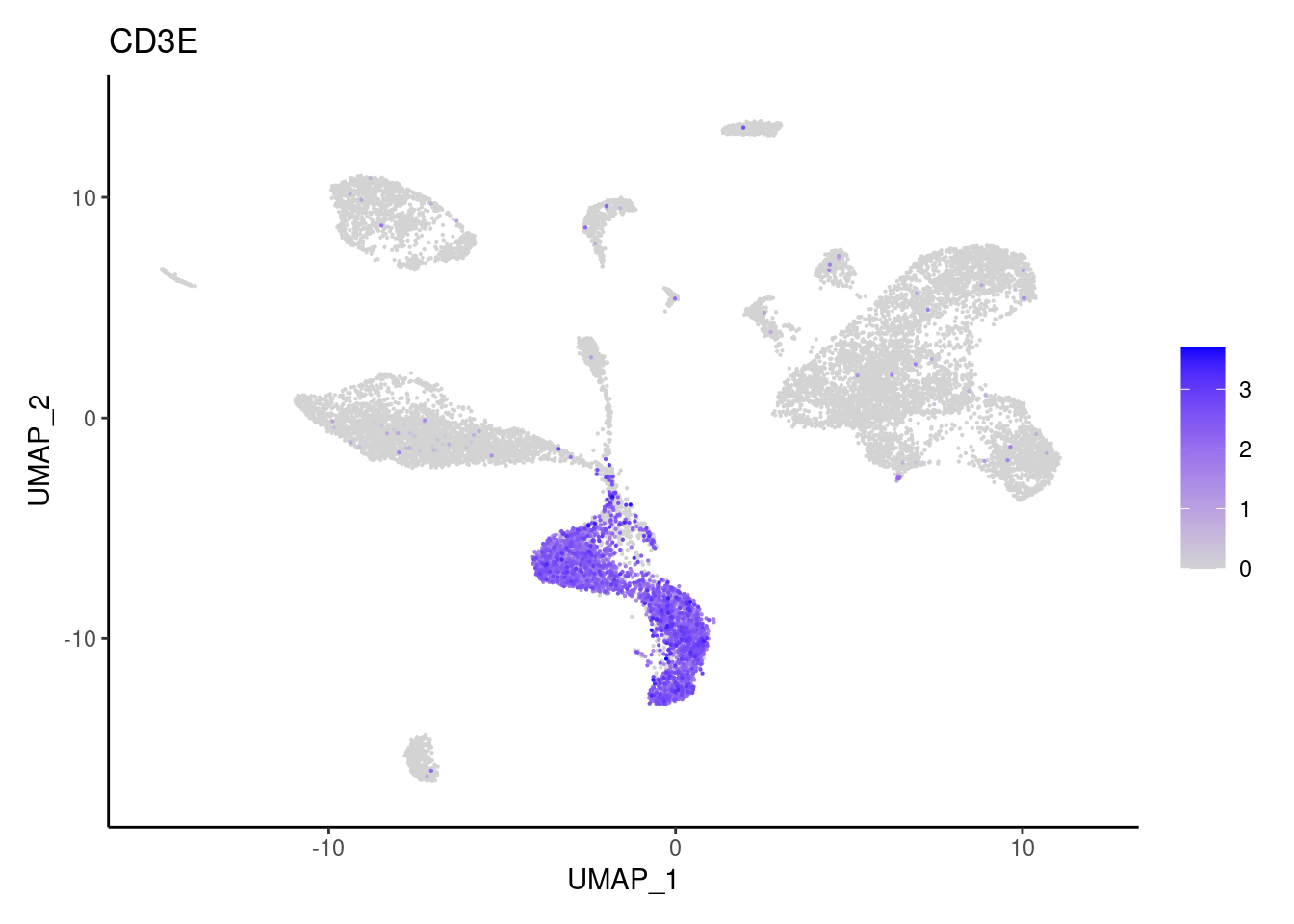
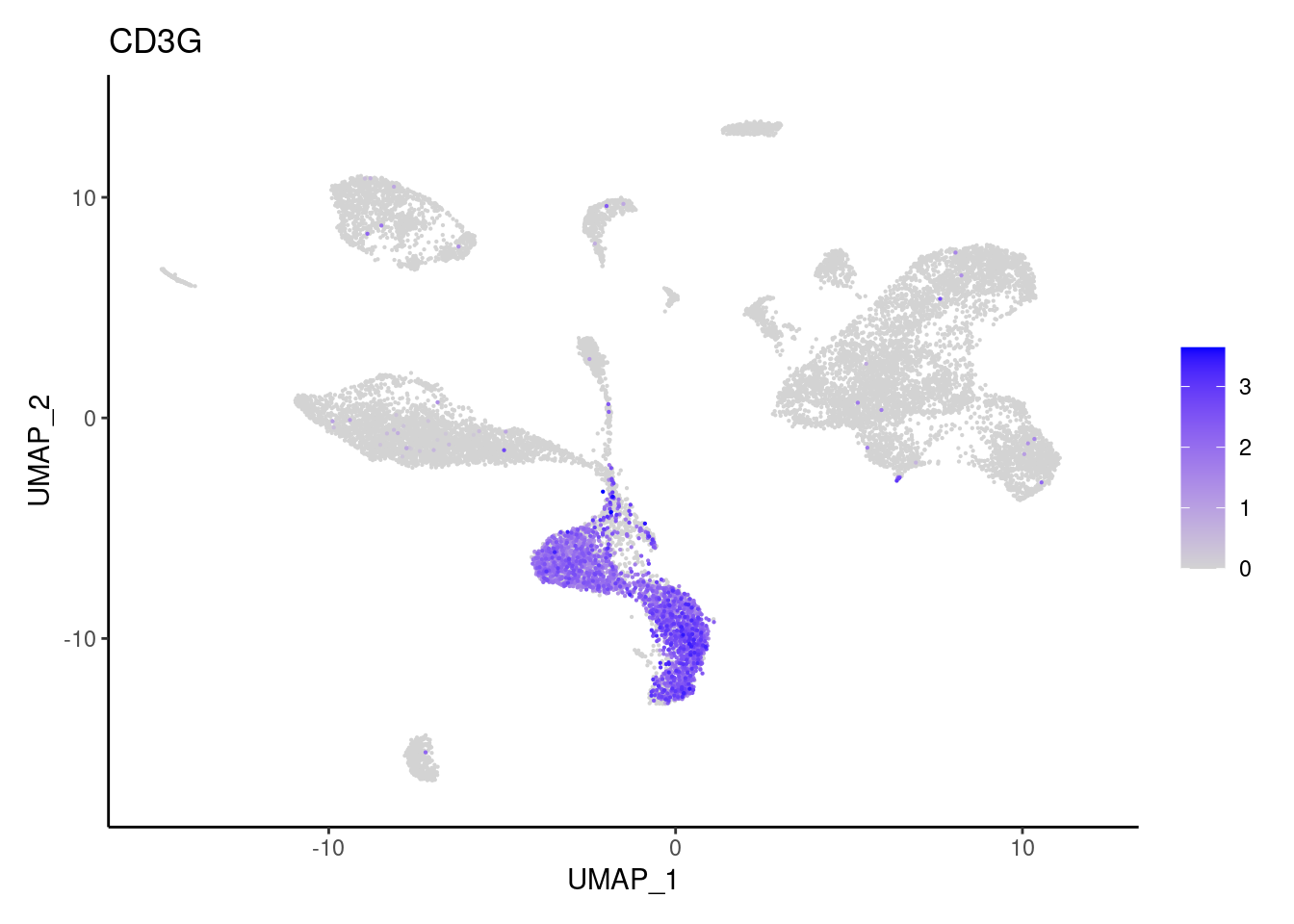
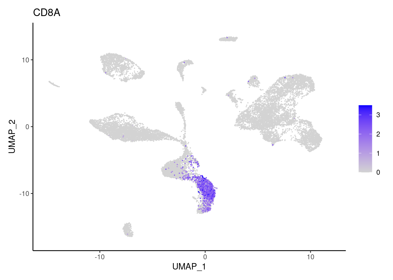
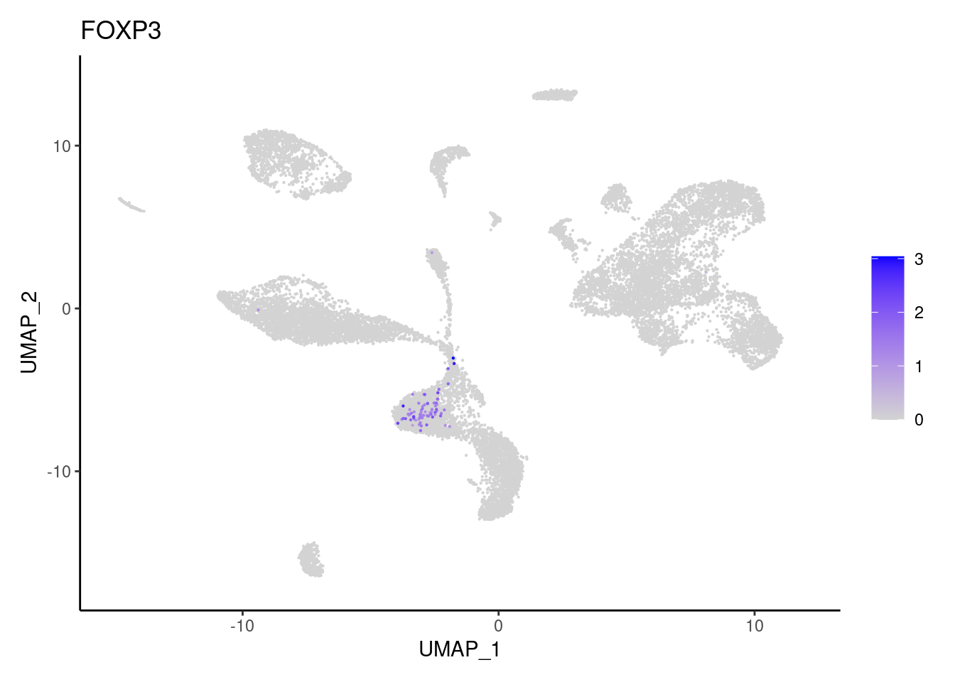
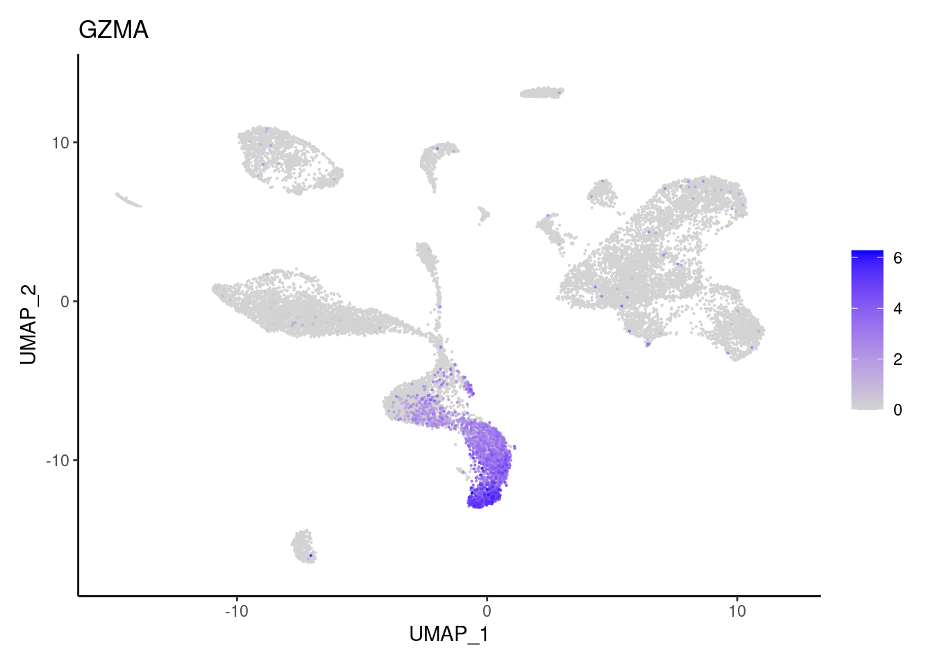
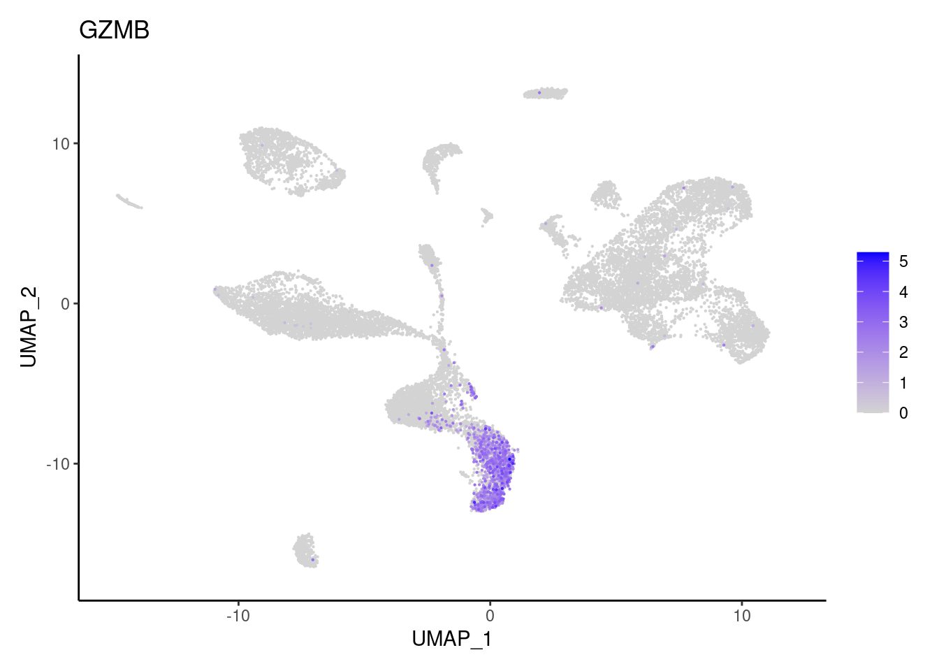
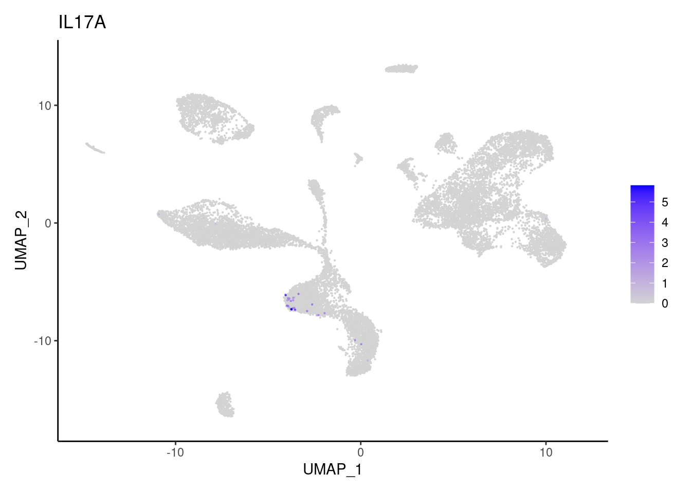
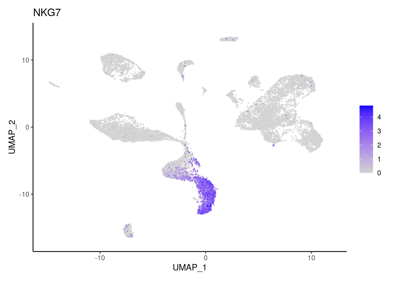
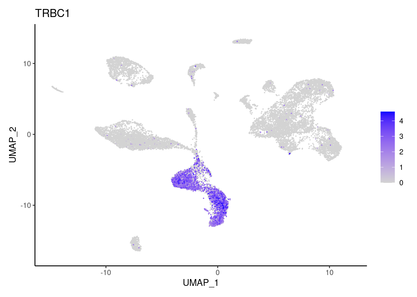
Previous knowledge genes
subset_genes <- data.frame(
  stringsAsFactors = FALSE,
                              gene = c("BANK1","CD19","CD79A","DERL3",
                                       "MS4A1","MZB1",
                                       "AQP8","BEST4", "EPCAM","MUC2",
                                       "OLFM4","PLCG2","TRPM5", "ZG16",
                                       "AIF1","C1QA","C1QB","CD14",
                                       "CMTM2","FCGR3B","LYZ","MS4A2",
                                       "TPSAB1","TPSB2","ACTA2","ADAMDEC1","CHI3L1",
                                       "COL3A1","NRXN1","PLVAP","SOX6",
                                       "VWF","CD3D","CD3E","CD3G",
                                       "CD8A","FOXP3","GZMA","GZMB",
                                       "IL17A","NKG7","TRBC1"),
                            subset = c("B and plasmacells","B and plasmacells",
                                       "B and plasmacells",
                                       "B and plasmacells","B and plasmacells",
                                       "B and plasmacells",
                                       "Epithelium","Epithelium",
                                       "Epithelium","Epithelium",
                                       "Epithelium","Epithelium",
                                       "Epithelium","Epithelium",
                                       "Myeloid cells","Myeloid cells",
                                       "Myeloid cells","Myeloid cells","Myeloid cells",
                                       "Myeloid cells","Myeloid cells",
                                       "Myeloid cells","Myeloid cells","Myeloid cells",
                                       "Stromal cells","Stromal cells",
                                       "Stromal cells","Stromal cells",
                                       "Stromal cells","Stromal cells","Stromal cells",
                                       "Stromal cells","T cells",
                                       "T cells","T cells","T cells",
                                       "T cells","T cells","T cells","T cells",
                                       "T cells","T cells")
                )
for(subset in unique(subset_genes$subset)){
  cat("### ", subset, "{.tabset} \n\n")
  genes <- subset_genes$gene[subset_genes$subset == subset]
  for (gene in genes) {
    j <- FeaturePlot(seudataf, features = gene, order=T) + theme_classic()
    cat("#### ", gene, "\n"); print(j); cat("\n\n")

  }
}
B and plasmacells
BANK1
CD19
CD79A
DERL3
MS4A1
MZB1
Epithelium
AQP8
BEST4
EPCAM
MUC2
OLFM4
PLCG2
TRPM5
ZG16
Myeloid cells
AIF1
C1QA
C1QB
CD14
CMTM2
FCGR3B
LYZ

MS4A2

TPSAB1

TPSB2

Stromal cells
ACTA2
ADAMDEC1
CHI3L1
COL3A1
NRXN1

PLVAP
SOX6
VWF
T cells
CD3D
CD3E
CD3G
CD8A
FOXP3
GZMA
GZMB
IL17A
NKG7
TRBC1
cat("## Dotplot of previous knowledge genes: \n")Dotplot of previous knowledge genes:
DotPlot(seudataf, features = subset_genes$gene, group.by = 'RNA_snn_res.0.1' ) + theme_classic() + theme(axis.text.x = element_text(angle=90, vjust = 0.5), axis.title = element_blank()) + NoLegend() + labs(title = 'Resolution 0.1')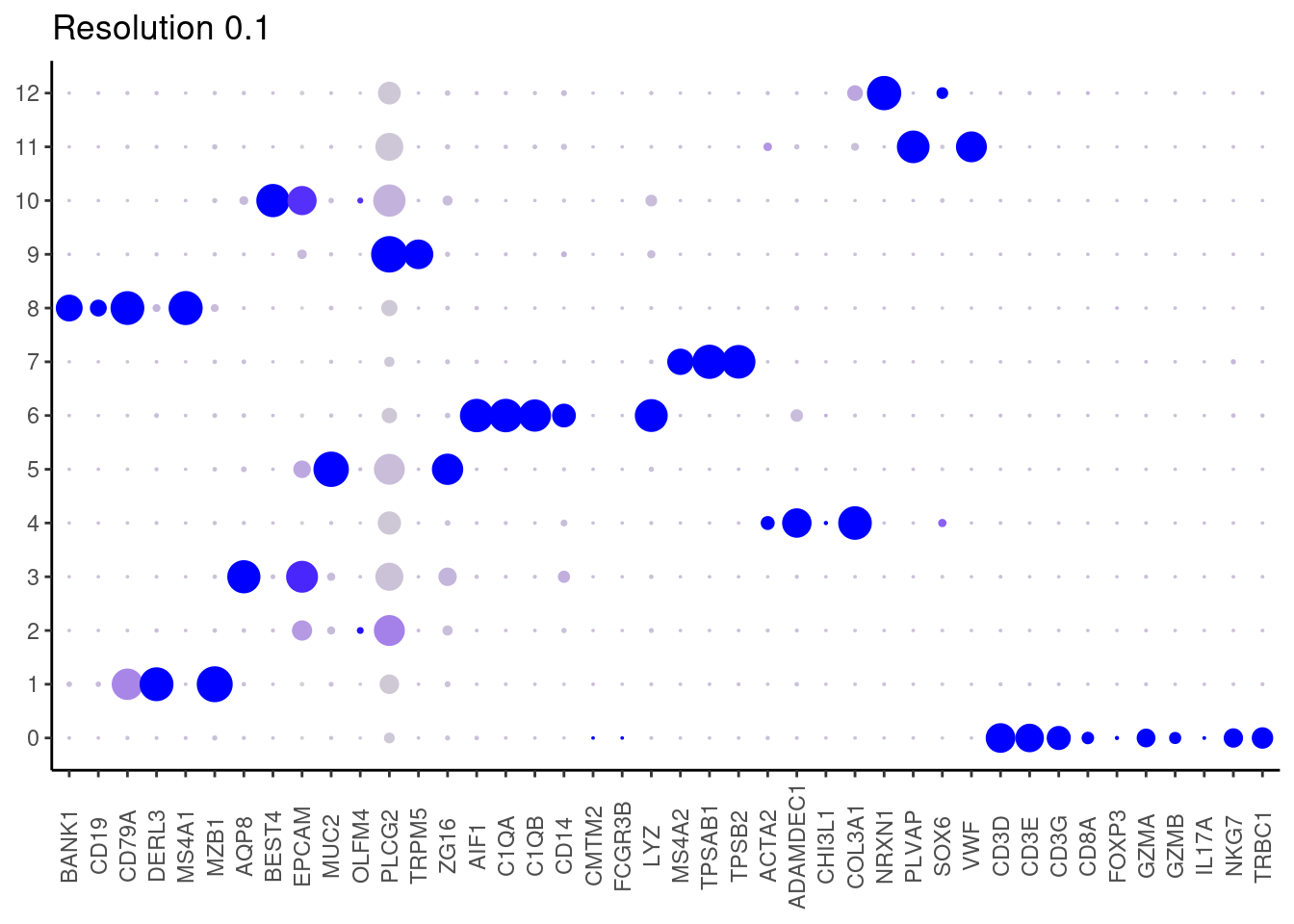
Subset annotation
anotation <- data.frame(cluster = 0:12,
                        anotation = c('tcells',#0
                                      'plasmas', #1
                                      'epi', #2
                                      'epi', #3
                                      'stroma', # 4
                                      'epi', # 5
                                      'myeloids', # 6
                                      'myeloids', # 7
                                      'plasmas', # 8
                                      'epi', # 9
                                      'epi', # 10
                                      'stroma', # 11
                                      'stroma' # 12
                        ))
seudataf$subset <- mapvalues(x = seudataf$RNA_snn_res.0.1,
                              from = anotation$cluster,
                              to = anotation$anotation)
DimPlot(seudataf, group.by = 'subset', label=T, cols = colors_subset)
tcells <- seudataf[,seudataf$subset == 'tcells']
plasmas <- seudataf[,seudataf$subset == 'plasmas']
myeloids <-seudataf[,seudataf$subset == 'myeloids']
epi <- seudataf[,seudataf$subset == 'epi']
stroma <- seudataf[,seudataf$subset == 'stroma']saveRDS(seudataf,'HC/filter_65/HC.RDS')
saveRDS(tcells, 'HC/tcells.RDS')
saveRDS(plasmas, 'HC/plasmas.RDS')
saveRDS(myeloids, 'HC/myeloids.RDS')
saveRDS(epi, 'HC/epi.RDS')
saveRDS(stroma, 'HC/stroma.RDS')Subset analysis
B and plasma cells
MT-gene expression
Distribution of cells in scatter plot (nfeatures/percent.mt) to check where are the majority of our cells. We can see the dots colored by density using the function get_density shown in Load extra functions and sources.
plasmas <- readRDS('HC/plasmas.RDS')
meta <- plasmas@meta.data
meta$density <- get_density(meta$percent.mt, meta$nFeature_RNA, n = 1000)
ggplot(meta) +
  geom_point(aes(percent.mt, nFeature_RNA, color = density), size = 0.2) +
  scale_color_viridis() + theme_classic() +
  scale_y_sqrt()+ scale_x_sqrt(breaks = c(1,10,100), limits = c(0,100))+
  geom_vline(xintercept = 25, linetype = 2, color = 'darkgray')+
  theme(text = element_text( size = 12),
        axis.title = element_text( size = 12),
        legend.text = element_blank())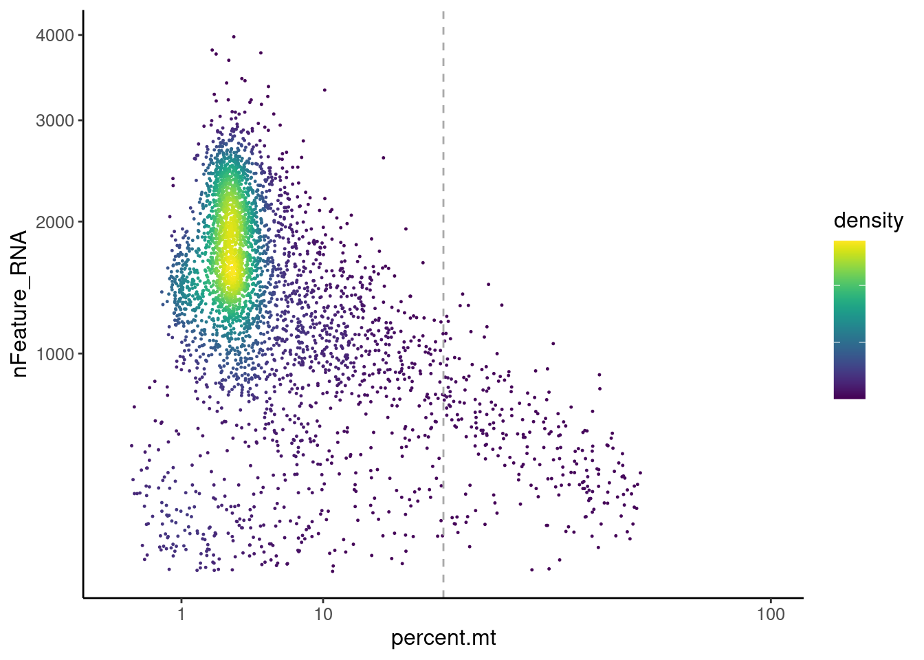
We analyzed the data using different cutoffs for the percent.mt (data not shown) and finally decided that 25% was a reasonable choice for our dataset.
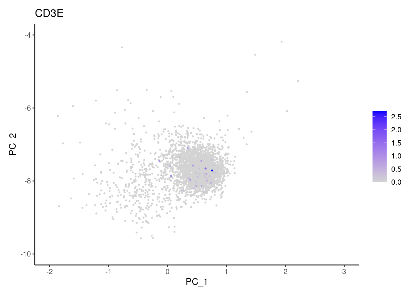
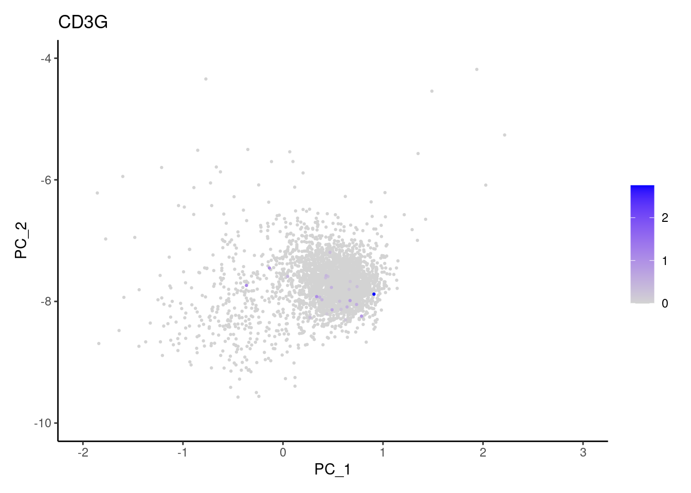
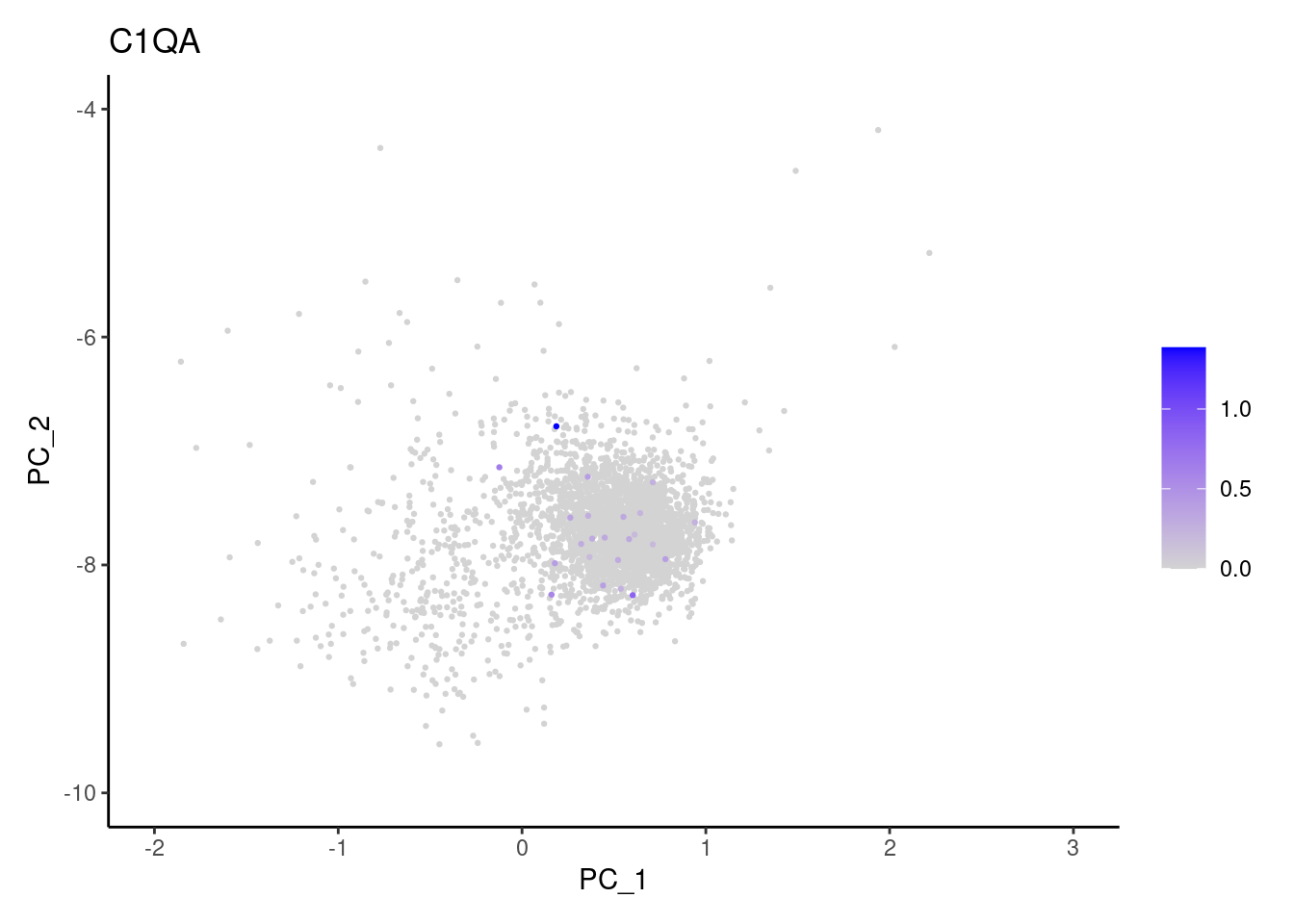
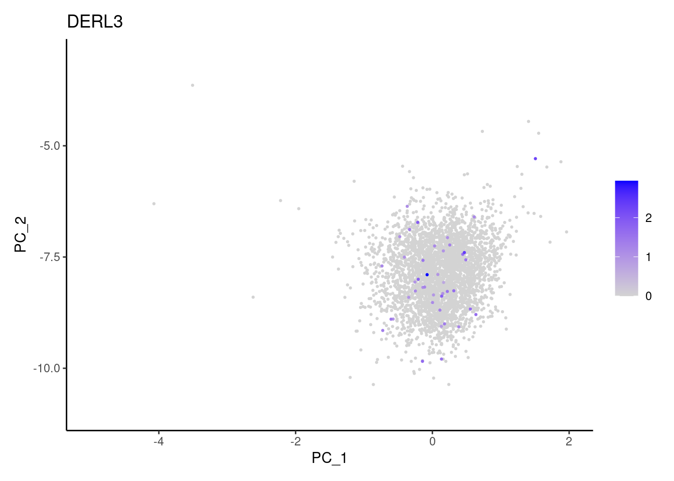
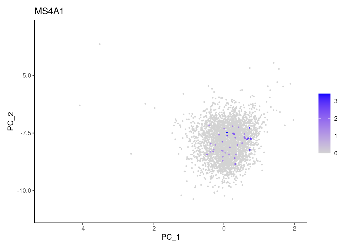
plasmas <- plasmas[,plasmas$percent.mt < 25]Non-B or Plasmacell genes
Right now plasmas has 3213 cells. Nevertheless, many
cells express genes that we know should not be expressed by B or
plasmacells. We will remove those cells.
genes <-  c('CD3E','CD3D','CD3G','C1QA','EPCAM')
for (gene in genes) {
    k <- FeaturePlot(plasmas, features = gene, order = T, reduction = 'pca')+
      theme_classic()
    cat("#### ", gene, "\n"); print(k); cat("\n\n")
  }
CD3E
CD3D

CD3G
C1QA
EPCAM
cat("#### code removal \n")code removal
counts <- plasmas@assays$RNA@counts
p <- grep("CD3E$|CD3D$|CD3G$|^C1QA$|^EPCAM$",rownames(plasmas))
pp <- which(Matrix::colSums(counts[p,])>0)
xx <-setdiff(colnames(plasmas), names(pp))
plasmas <- subset(plasmas,cells = xx)
cat('\n\n')
Genes wo expression
We remove the genes without expression from the dataset.
counts <- plasmas@assays$RNA@counts
pp <- which(Matrix::rowSums(counts)==0)
xx <-setdiff(rownames(plasmas), names(pp))
plasmas <- subset(plasmas, features = xx)
Dimension reduction
plasmas <- seurat_to_pca(plasmas)
## [1] "NORMALIZATION"
## [1] "VARIABLE FEATURES"
## [1] "SCALE DATA"
## [1] "RUN PCA"

a <- ElbowPlot(plasmas, ndims = 100) +
  geom_vline(xintercept = 25, colour="#BB0000", linetype = 2)+
  labs(title = paste0('Elbowplot')) + theme_classic()

plasmas<- FindNeighbors(plasmas, dims = 1:25)
plasmas<-RunUMAP(plasmas, dims=1:25)
b <- DimPlot(plasmas, group.by = 'sample_name') +
  labs(title = '25 PCS') +
  theme_classic() +
  theme(legend.position = 'bottom')

(a+b) / guide_area() +
  plot_layout(heights = c(0.7,0.3),guides = 'collect')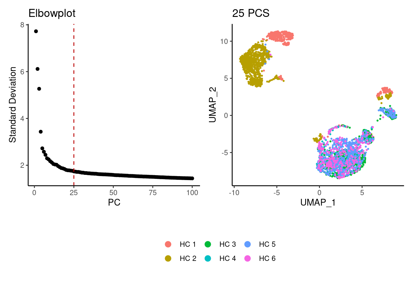
Harmony correction:
plasmas <- RunHarmony(plasmas, group.by = 'sample_name', dims.use = 1:25)
a <- ElbowPlot(plasmas, ndims = 100, reduction = 'harmony') +
  geom_vline(xintercept = 30, linetype = 2) +
  labs(title = paste0('Harmony - 25PCS'))
plasmas<- FindNeighbors(plasmas, reduction = "harmony", dims = 1:30)
plasmas<-RunUMAP(plasmas, dims=1:30, reduction= "harmony")

b <- DimPlot(plasmas, group.by = 'sample_name') + labs(title = 'B cells and plasmas - Harmony 25-30')

a + b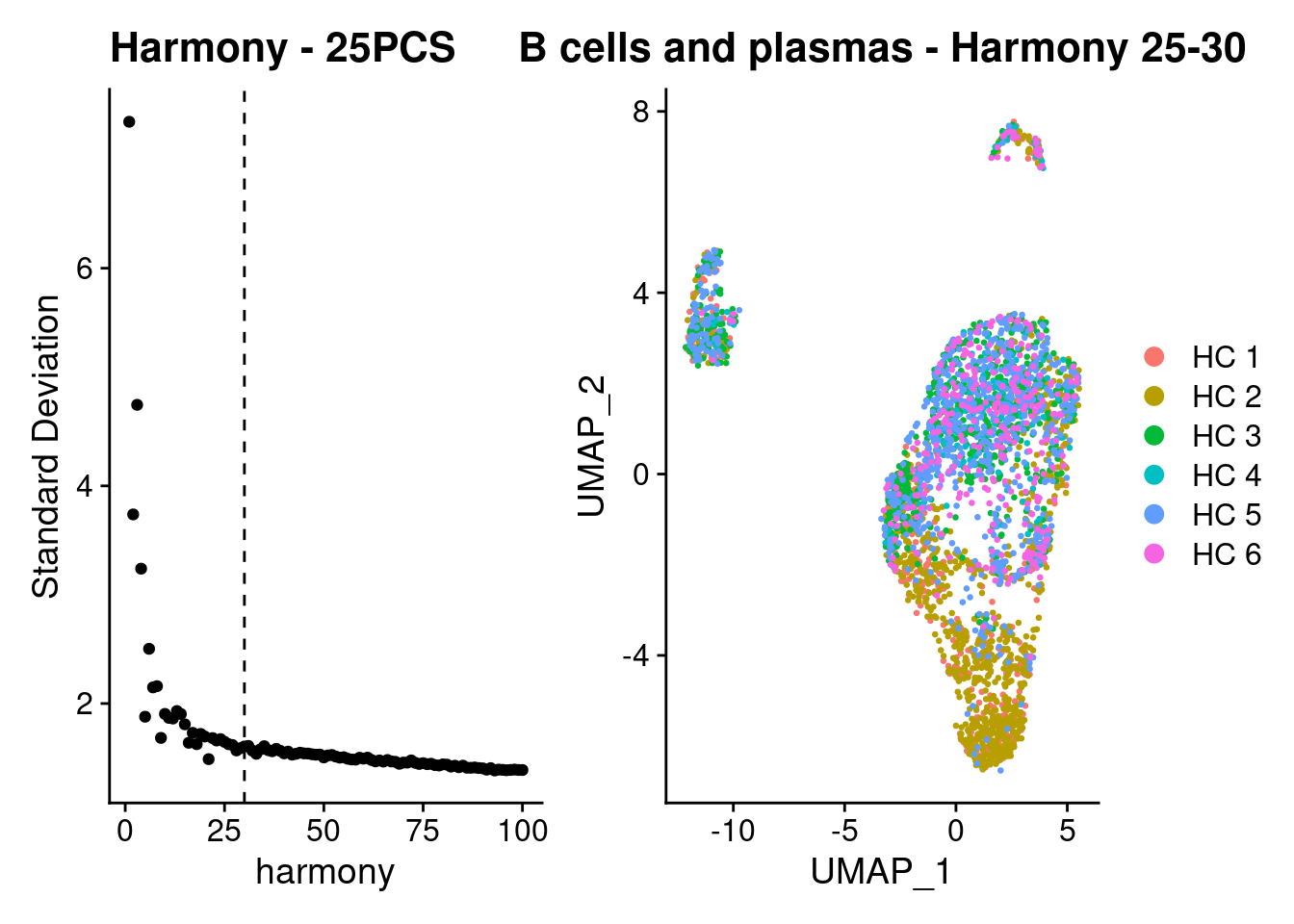
Louvain clusterization
dir.create('HC/plasmas/')
dir.create('HC/plasmas/plasmas_harmony_25_30/')
plasmas <- resolutions(plasmas,
                       workingdir = 'HC/plasmas/plasmas_harmony_25_30/',
                       title = 'plasmas_harmony_25_30')
saveRDS(plasmas, file = 'HC/plasmas/plasmas_harmony_25_30/plasmas_filtered_25_30.RDS')
clustree::clustree(plasmas, prefix = 'RNA_snn_res.')
clustree::clustree(plasmas, prefix = 'RNA_snn_res.')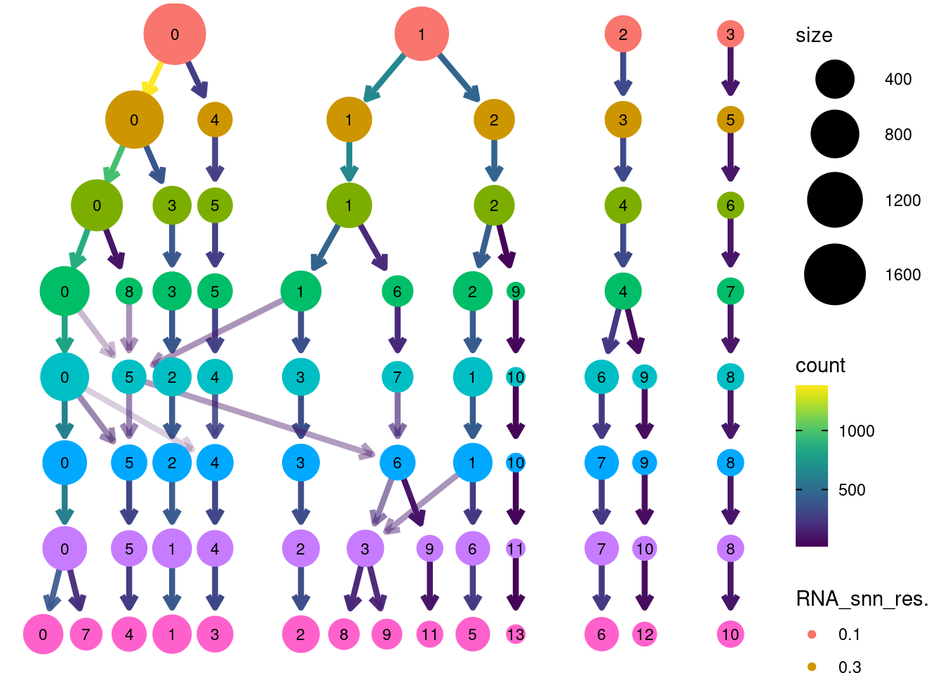
Annotation
plasmas$annotation <- plyr::mapvalues(x = plasmas$RNA_snn_res.0.9,
                                      from = 0:10,
                                      to = c("PC IgA",
                                             "PC IgA",
                                             "Plasmablast IgA HS",
                                             "Plasmablast IER",
                                             "Plasmablast IGLL5 IgA",
                                             "B cell",
                                             "PC IgA",
                                             "Plasmablast IgG",
                                             "B cell GC",
                                             "Plasmablast low genes",
                                             "PC IgA"))

DimPlot(plasmas, group.by = 'annotation') 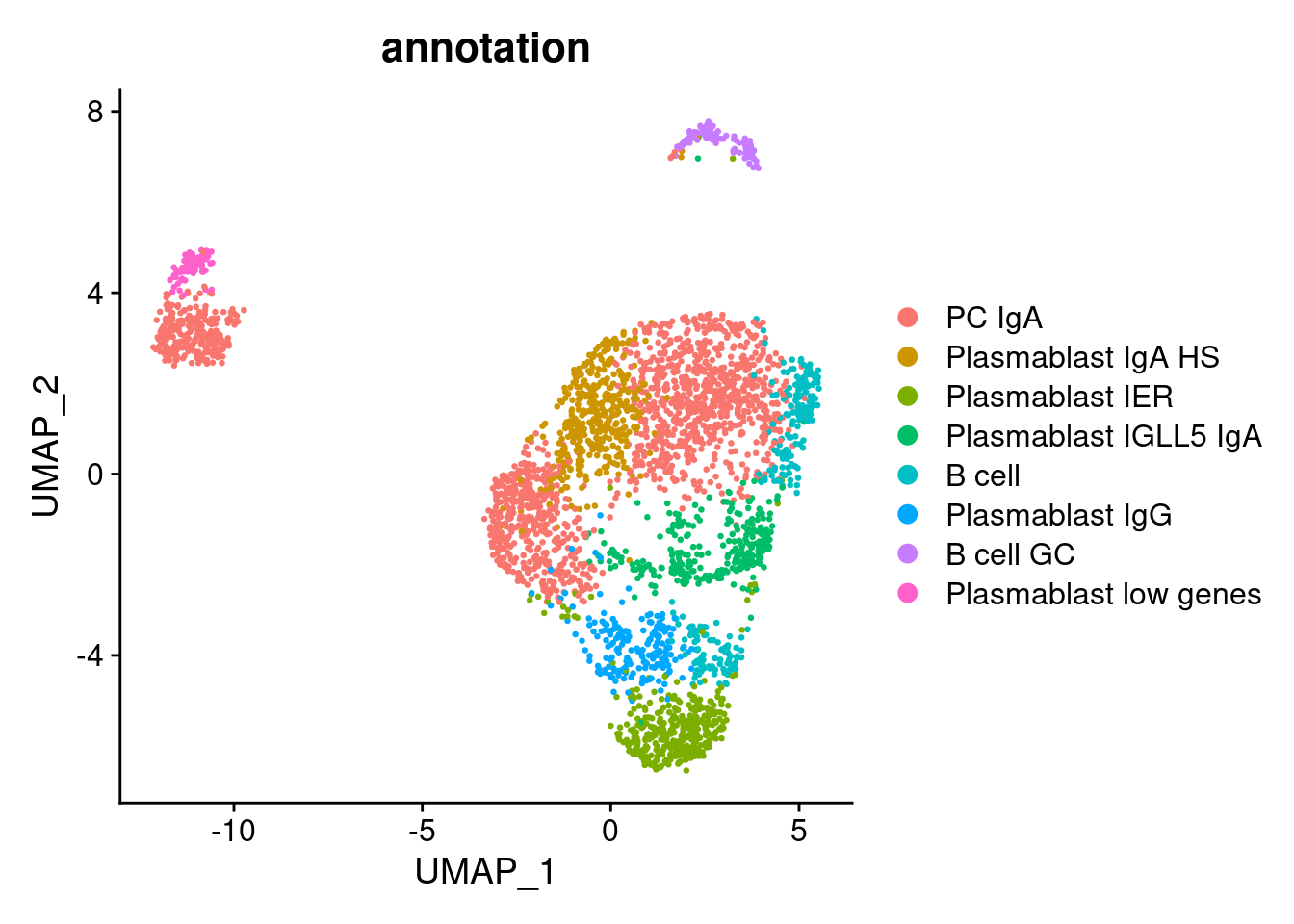
dir.create('HC/annotated')
saveRDS(plasmas, file = 'HC/annotated/plasmas.RDS')
T cells
MT-gene expression
Distribution of cells in scatter plot (nfeatures/percent.mt) to check where are the majority of our cells. We can see the dots colored by density using the function get_density shown in Load extra functions and sources.
tcells <- readRDS('HC/tcells.RDS')
meta <- tcells@meta.data
meta$density <- get_density(meta$percent.mt, meta$nFeature_RNA, n = 100)
ggplot(meta) +
  geom_point(aes(percent.mt, nFeature_RNA, color = density), size = 0.2) +
  scale_color_viridis() + theme_classic() +
  scale_y_log10()+
  geom_vline(xintercept = 25, linetype = 2, color = 'gray')+
  theme(text = element_text( size = 12),
        axis.title = element_text( size = 12),
        legend.text = element_blank())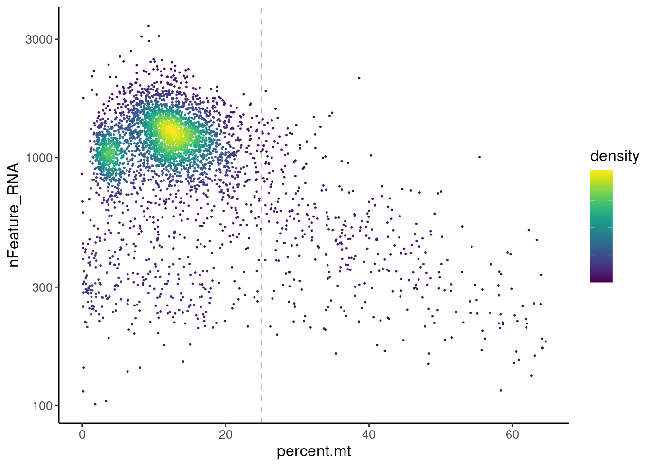
We analyzed the data using different cutoffs for the percent.mt (data not shown) and finally decided that 25% was a reasonable choice for our dataset.
tcells <- tcells[,tcells$percent.mt < 25]Non-T cell genes
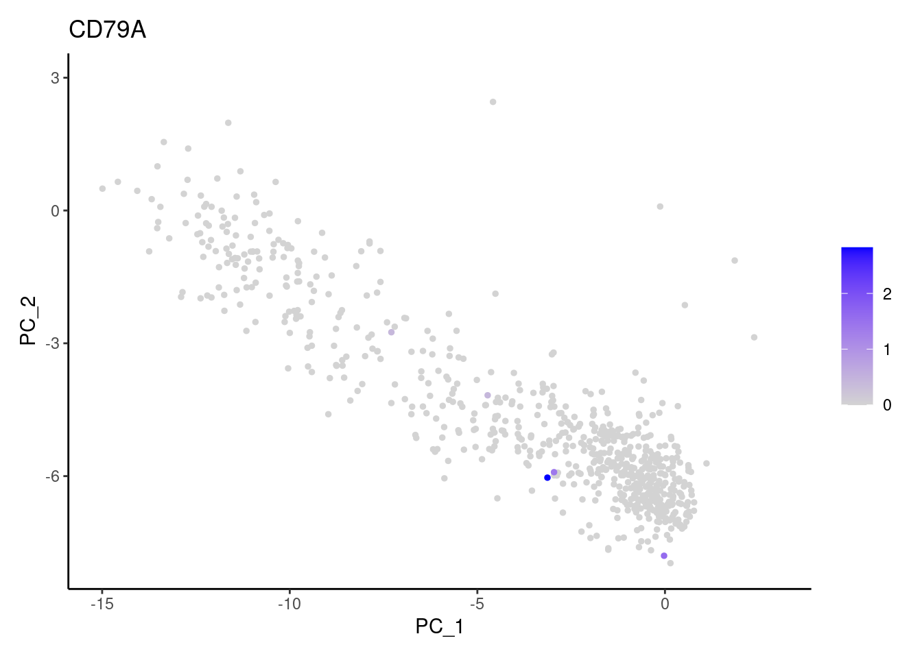
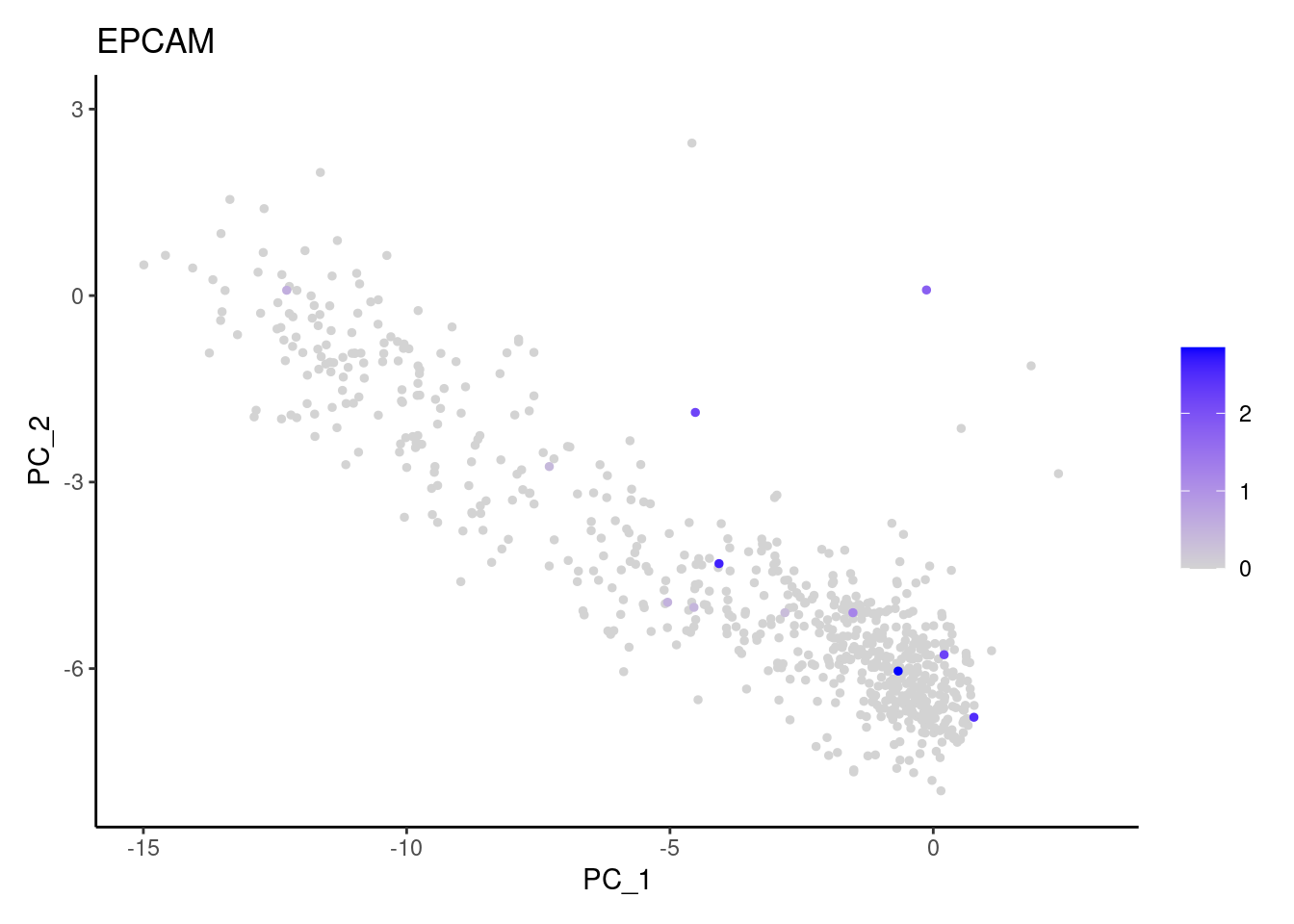
Right now tcells has 3482 cells. Nevertheless, many
cells express genes that we know should not be expressed by T cells. We
will remove those cells.
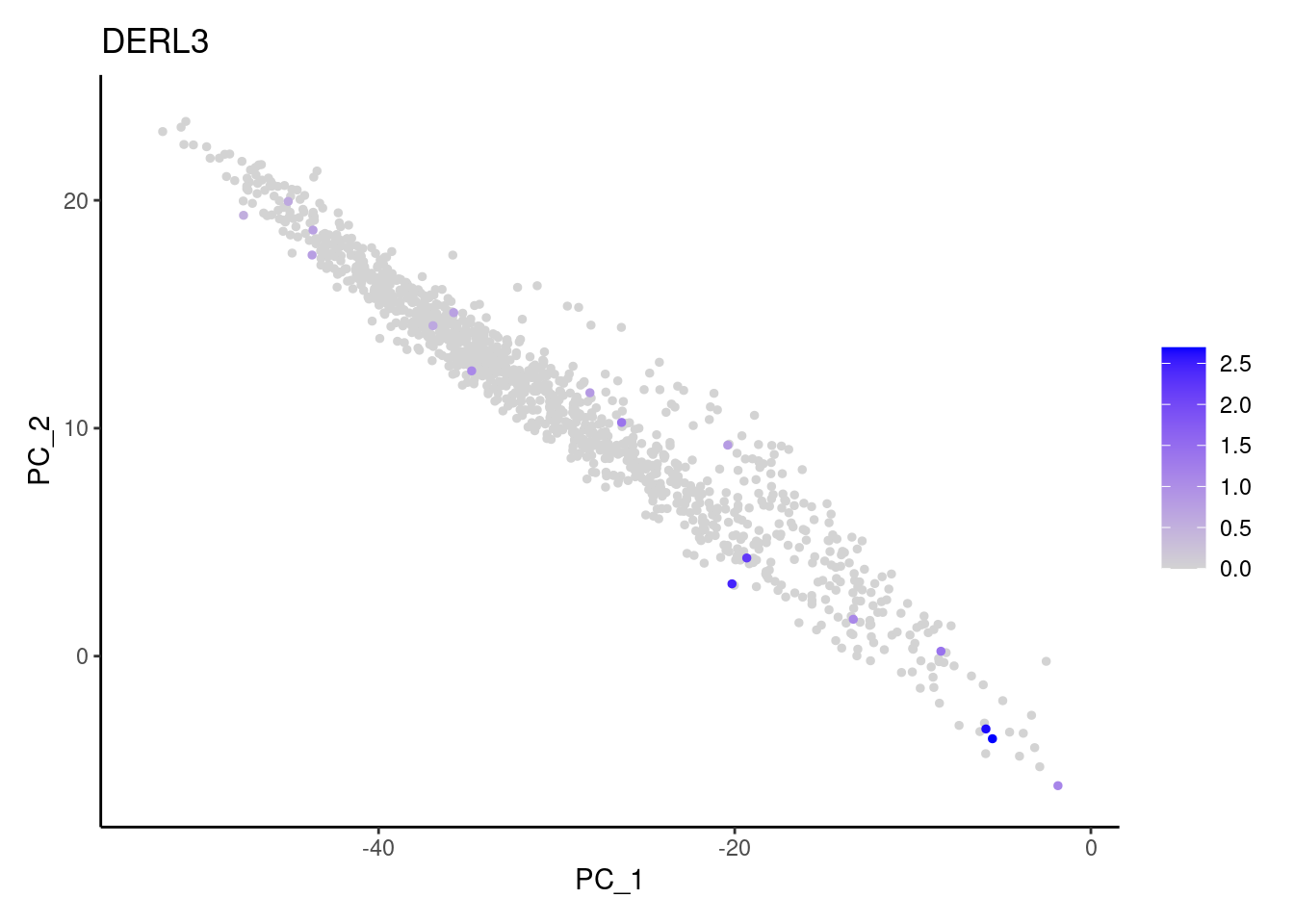
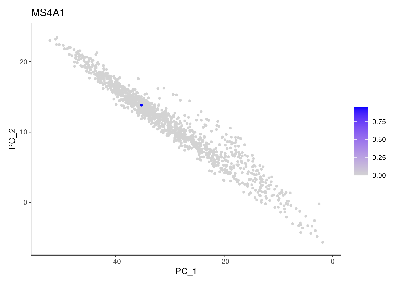
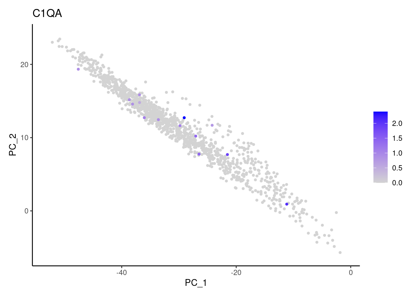
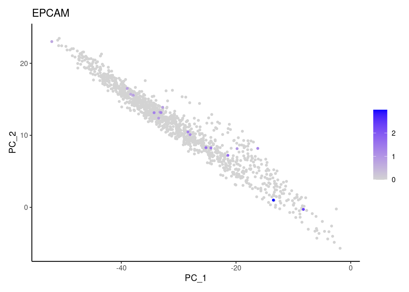
genes <-  c('DERL3', 'MS4A1', 'C1QA', 'EPCAM', 'CD79A')
for (gene in genes) {
     k <- FeaturePlot(tcells, features = gene, order = T, reduction='pca')+
      theme_classic()
    cat("#### ", gene, "\n"); print(k); cat("\n\n")
  }
DERL3
MS4A1
C1QA
EPCAM
CD79A

cat("#### code removal \n")code removal
counts <- tcells@assays$RNA@counts
p <- grep("^DERL3$|^MS4A1$|^C1QA$|^EPCAM$|^CD79A$",rownames(tcells))
pp <- which(Matrix::colSums(counts[p,])>0)
xx <-setdiff(colnames(tcells), names(pp))
tcells <- subset(tcells,cells = xx)
cat('\n\n')
Ig genes signal
We have observed that due to normalization, there’s high Ig gene expression in cells that did not have high counts of Ig genes. As an example:
kd <- FeaturePlot(tcells, features = 'IGHA1', slot = 'data', order = T) + labs(title = 'data')
kc <- FeaturePlot(tcells, features = 'IGHA1', slot = 'counts', order = T)+ labs(title = 'counts')

wrap_plots(kc,kd, nrow = 1)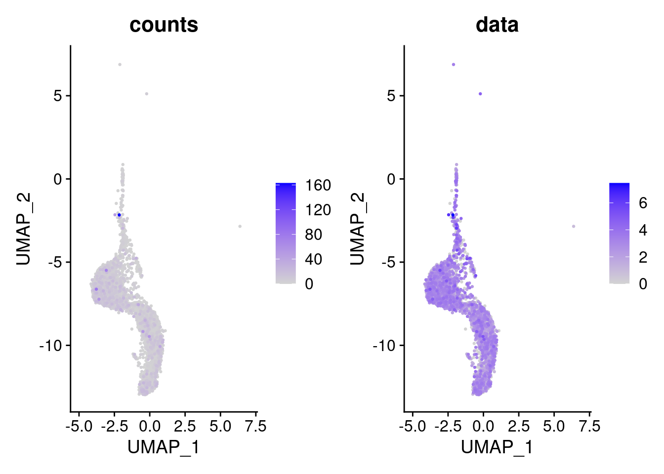
We remove the Ig genes from the dataset in all subsets except for the plasma and B cells subset.
gg <- rownames(tcells)[c(grep("^IGH",rownames(tcells)),
                         grep("^IGK", rownames(tcells)),
                         grep("^IGL", rownames(tcells)))]
genes <- setdiff(rownames(tcells),gg)
tcells <- subset(tcells,features = genes)
Genes wo expression
We remove the genes without expression from the dataset.
counts <- tcells@assays$RNA@counts
pp <- which(Matrix::rowSums(counts)==0)
xx <-setdiff(rownames(tcells), names(pp))
tcells <- subset(tcells, features = xx)
Dimension reduction
We tried different values of PC for the UMAP generation and Louvain clusterization. Finally, we considered 25 PCs for the analysis.
tcells <- seurat_to_pca(tcells)

a <- ElbowPlot(tcells, ndims = 100) +
  geom_vline(xintercept = 25, colour="#BB0000", linetype = 2)+
  labs(title = paste0('Elbowplot')) + theme_classic()

tcells<- FindNeighbors(tcells, dims = 1:25)
tcells<-RunUMAP(tcells, dims=1:25)
b <- DimPlot(tcells, group.by = 'sample_name') +
  labs(title = '25 PCS') +
  theme_classic() +
  theme(legend.position = 'bottom')

(a+b) / guide_area() +
  plot_layout(heights = c(0.7,0.3),guides = 'collect')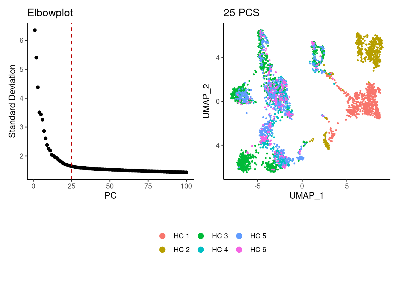
Harmony correction
tcells <- RunHarmony(tcells, group.by = 'sample_name', dims.use = 1:25)
a <- ElbowPlot(tcells, ndims = 100, reduction = 'harmony') +
  geom_vline(xintercept = 25, linetype = 2)
tcells<- FindNeighbors(tcells, reduction = "harmony", dims = 1:25)
tcells<-RunUMAP(tcells, dims=1:25, reduction= "harmony")

b <- DimPlot(tcells, group.by = 'sample_name') + theme_classic() +
  theme(legend.position = 'bottom')

(a+b) / guide_area() +
  plot_layout(heights = c(0.7,0.3),guides = 'collect')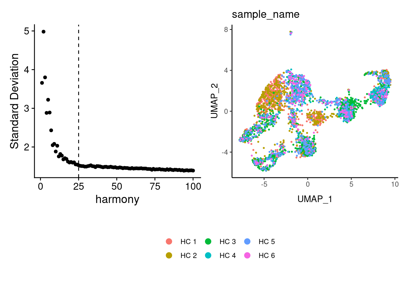
Louvain Clusterization
dir.create('HC/Tcells/')
path <- getwd()
tcells <- resolutions(tcells,
                   workingdir = path,
                   title = 'HC/Tcells/Markers_tcells_')
saveRDS(tcells, file = 'HC/Tcells/tcells_filtered.RDS')
clustree::clustree(tcells, prefix = 'RNA_snn_res.')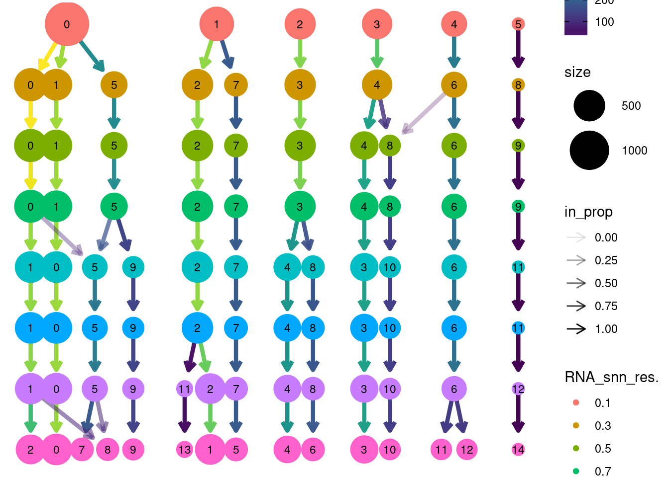
Annotation
tcells$annotation <- plyr::mapvalues(x = tcells$RNA_snn_res.1.5,
                                      from = 0:14,
                                      to = c("CD4 ANXA1",
                                             "CD8 CTL",
                                             "CD4 IER",
                                             "CD8 CTL",
                                             "IELs.1",
                                             "CD8 ZNF683",
                                             "IELs.2",
                                             "CD4 naïve",
                                             "Naïve Ribhi",
                                             "Tregs",
                                             "CD8 IER",
                                             "T cells Ribhi",
                                             "T cells MT",
                                             "T cells low genes",
                                             "ILC3"))

DimPlot(tcells, group.by = 'annotation') 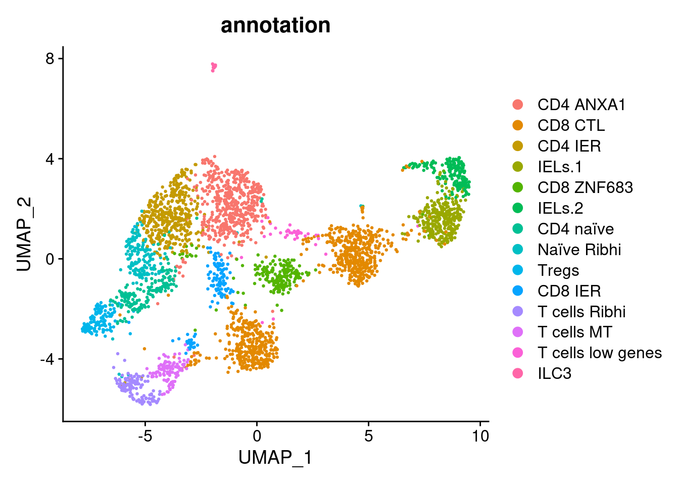
saveRDS(tcells, file = 'HC/annotated/tcells.RDS')Epithelial cells
MT-gene expression
Distribution of cells in scatter plot (nfeatures/percent.mt) to check where are the majority of our cells. We can see the dots colored by density using the function get_density shown in Load extra functions and sources.
epi <- readRDS('HC/epi.RDS')
meta <- epi@meta.data
meta$density <- get_density(meta$percent.mt, meta$nFeature_RNA, n = 100)
ggplot(meta) +
  geom_point(aes(percent.mt, nFeature_RNA, color = density), size = 0.2) +
  scale_color_viridis() + theme_classic() +
  scale_y_log10()+
  geom_vline(xintercept = 65, linetype = 2, color = 'gray')+
  theme(text = element_text( size = 12),
        axis.title = element_text( size = 12),
        legend.text = element_blank())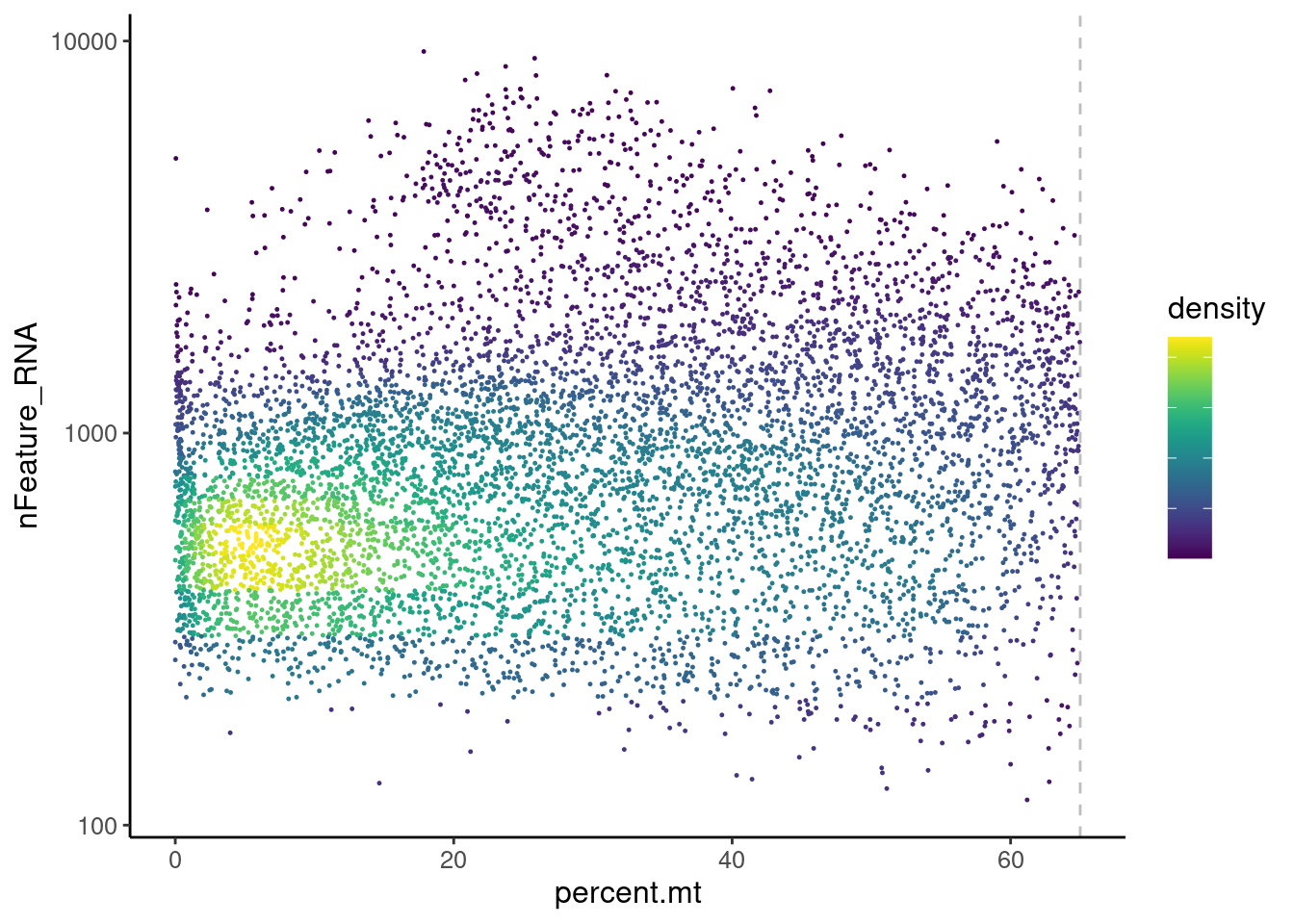
We analyzed the data using different cutoffs for the percent.mt (data not shown) and finally decided that 65% was a reasonable choice for this dataset.
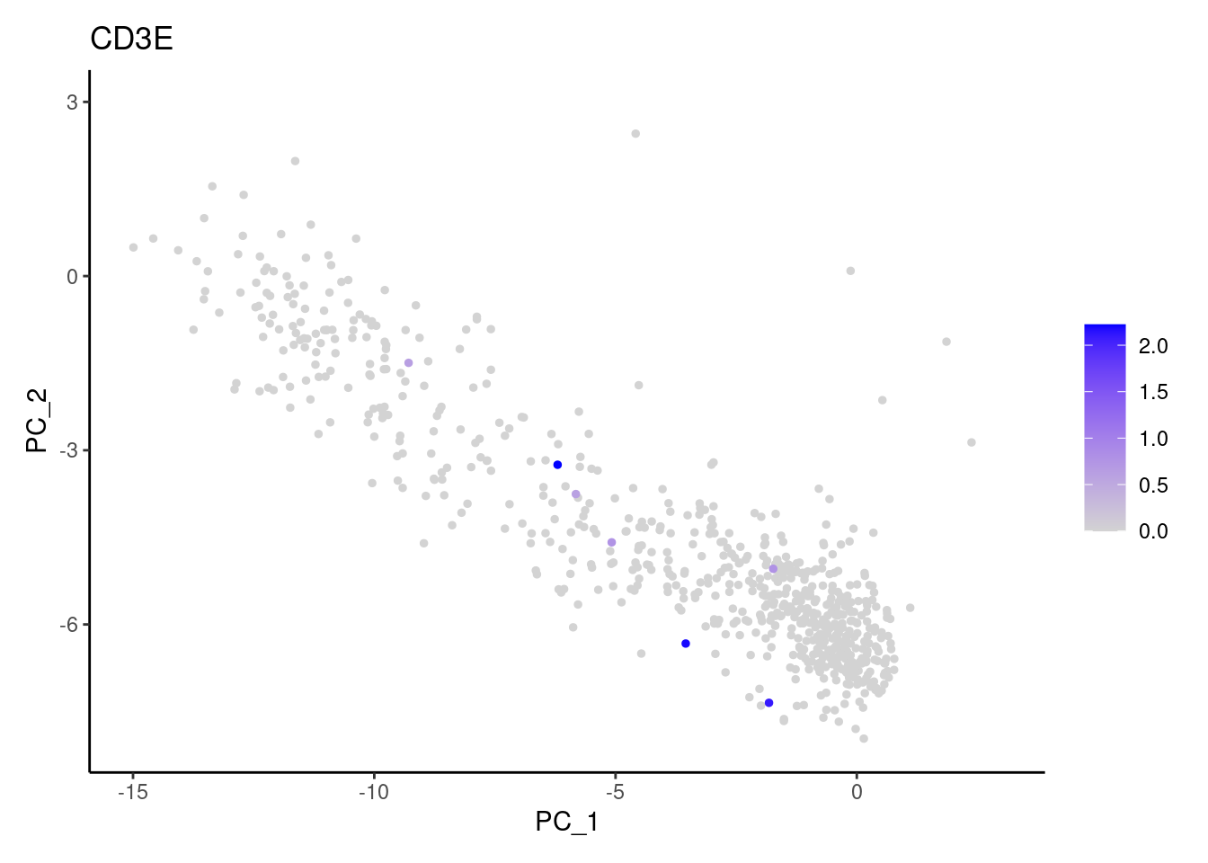
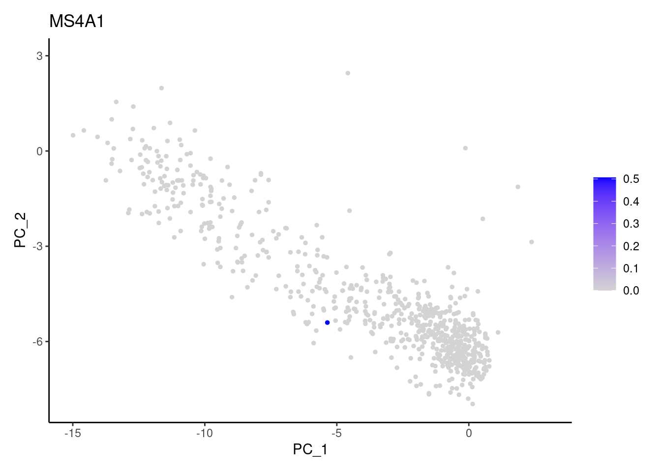
Non-epithelial genes
Right now epi has 6965 cells. Nevertheless, many cells
express genes that we know should not be expressed by epithelial cells.
We will remove those cells.
genes <-  c('CD3E','CD3D','CD3G', 'C1QA', 'DERL3', 'MS4A1', 'C1QA')
for (gene in genes) {
    j <- FeaturePlot(epi, features = gene, order=T, reduction = 'pca') + theme_classic()
    cat("#### ", gene, "\n"); print(j); cat("\n\n")
  }
CD3E

CD3D

CD3G

C1QA

DERL3
MS4A1

C1QA

cat("#### code removal \n")code removal
counts <- epi@assays$RNA@counts
p <- grep("CD3E$|CD3D$|CD3G$|MS4A1$|DERL3|^C1QA$",rownames(epi))
pp <- which(Matrix::colSums(counts[p,])>0)
xx <-setdiff(colnames(epi), names(pp))
epi <- subset(epi,cells = xx)
cat('\n\n')
Ig genes signal
We have observed that due to normalization, there’s high Ig gene expression in cells that did not have high counts of Ig genes. As an example:
a <- FeaturePlot(epi, features = 'IGHA1', slot = 'counts') + labs(title='counts') + theme_classic()
b <- FeaturePlot(epi, features = 'IGHA1', slot = 'data') + labs(title= 'data') + theme_classic()
wrap_plots(a,b, nrow = 1)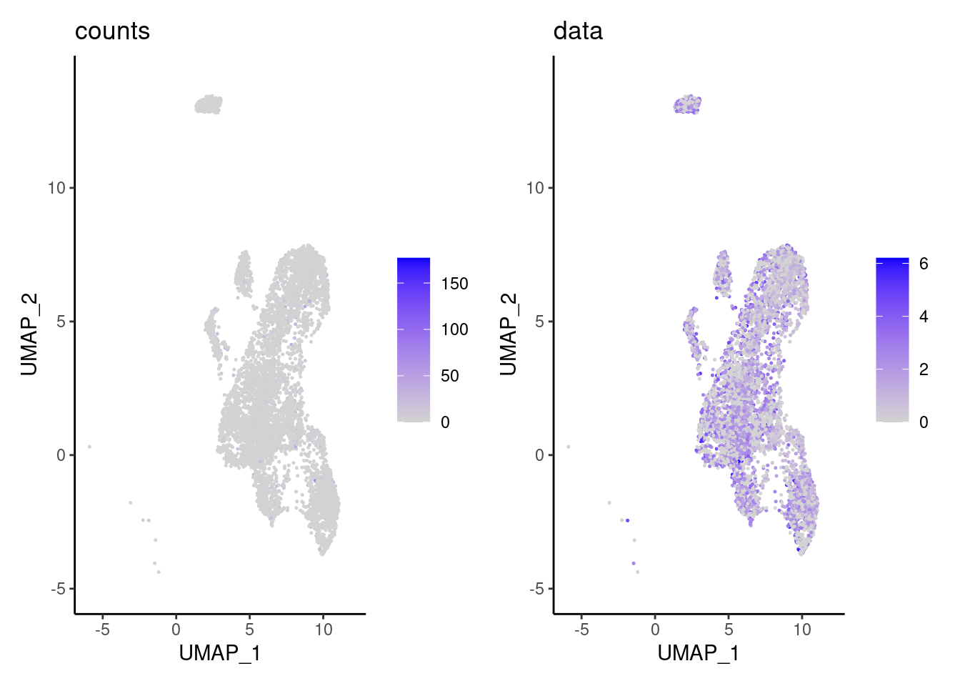
We remove the Ig genes from the dataset in all subsets except for the plasma and B cells subset.
gg <- rownames(epi)[c(grep("^IGH",rownames(epi)),
                         grep("^IGK", rownames(epi)),
                         grep("^IGL", rownames(epi)))]
genes <- setdiff(rownames(epi),gg)
epi <- subset(epi,features = genes)
Genes without expression
We remove the genes without expression from the dataset.
counts <- epi@assays$RNA@counts
pp <- which(Matrix::rowSums(counts)==0)
xx <-setdiff(rownames(epi), names(pp))
epi <- subset(epi, features = xx)
Dimension reduction
epi <- seurat_to_pca(epi)

a <- ElbowPlot(epi, ndims = 100) +
  geom_vline(xintercept = 27, colour="#BB0000", linetype = 2)+
  labs(title = paste0('Elbowplot')) + theme_classic()

epi<- FindNeighbors(epi, dims = 1:27)
epi<-RunUMAP(epi, dims=1:27)
b <- DimPlot(epi, group.by = 'sample_name') +
  labs(title = '27 PCS') +
  theme_classic() +
  theme(legend.position = 'bottom')

(a+b) / guide_area() +
  plot_layout(heights = c(0.7,0.3),guides = 'collect')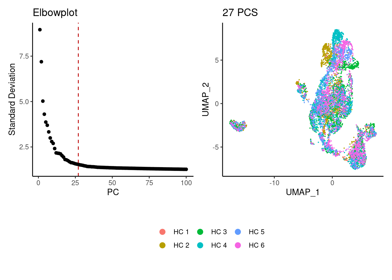
Louvain Clusterization
path <- getwd()
dir.create('HC/Epithelium')
epi <- resolutions(epi,
                   workingdir = path,
                   title = 'HC/Epithelium/Markers_Epithelium_')
saveRDS(epi, file = 'HC/Epithelium/epi_filtered.RDS')
clustree::clustree(epi, prefix = 'RNA_snn_res.')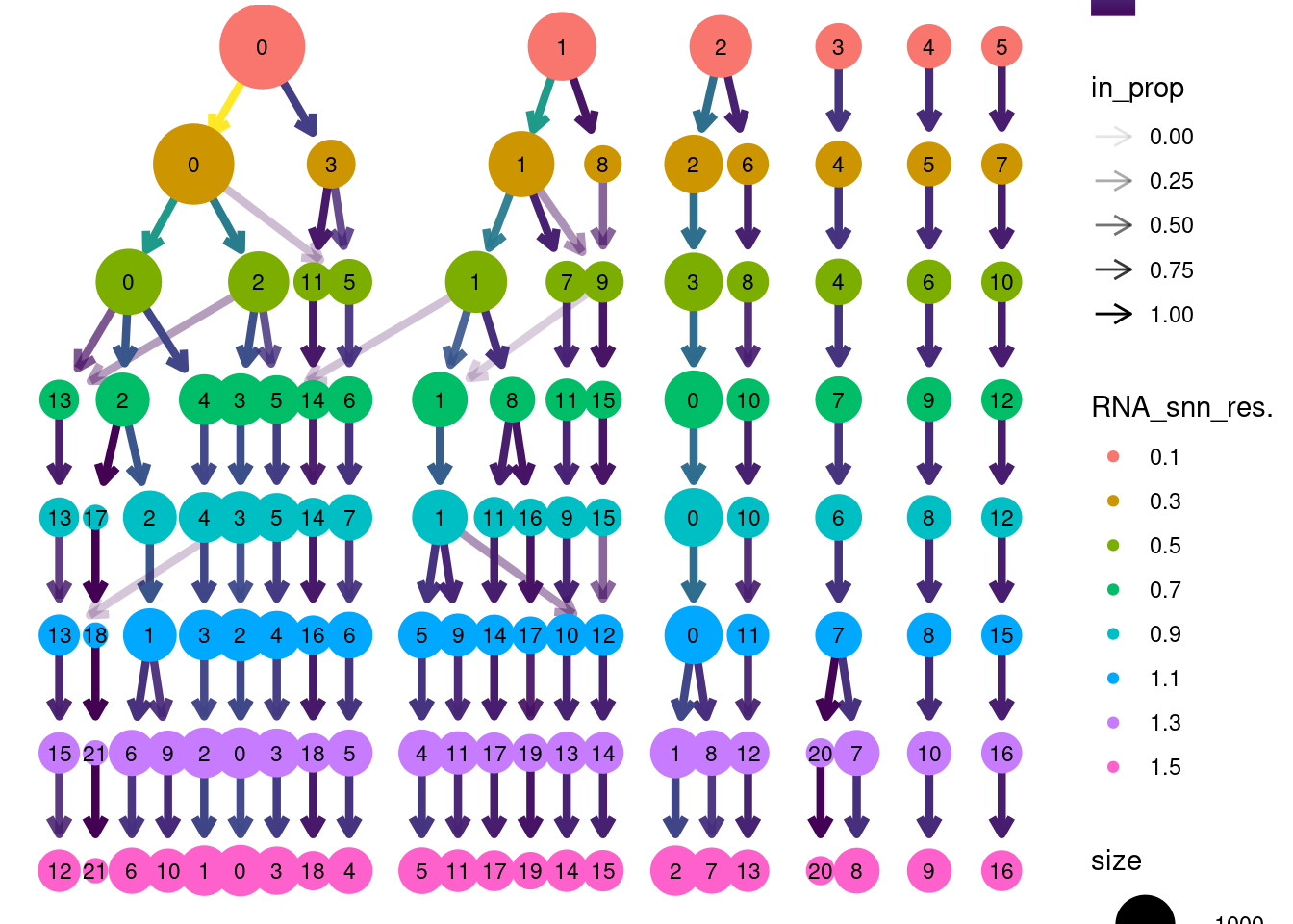
Annotation
epi$annotation <- plyr::mapvalues(x = epi$RNA_snn_res.0.5,
                                  from = 0:11,
                                  to = c("Epithelium Ribhi",
                                         "Colonocyte 1",
                                         "PLCG2 colonocyte",
                                         "Goblet",
                                         "Secretory progenitor",
                                         "Cycling TA",
                                         "Tuft cells",
                                         "Colonocyte 2",
                                         "Goblet mature",
                                         "Colonocyte APC",
                                         "BEST4 OTOP2",
                                         "Epithelium Ribhi 2"))

DimPlot(epi, group.by = 'annotation') 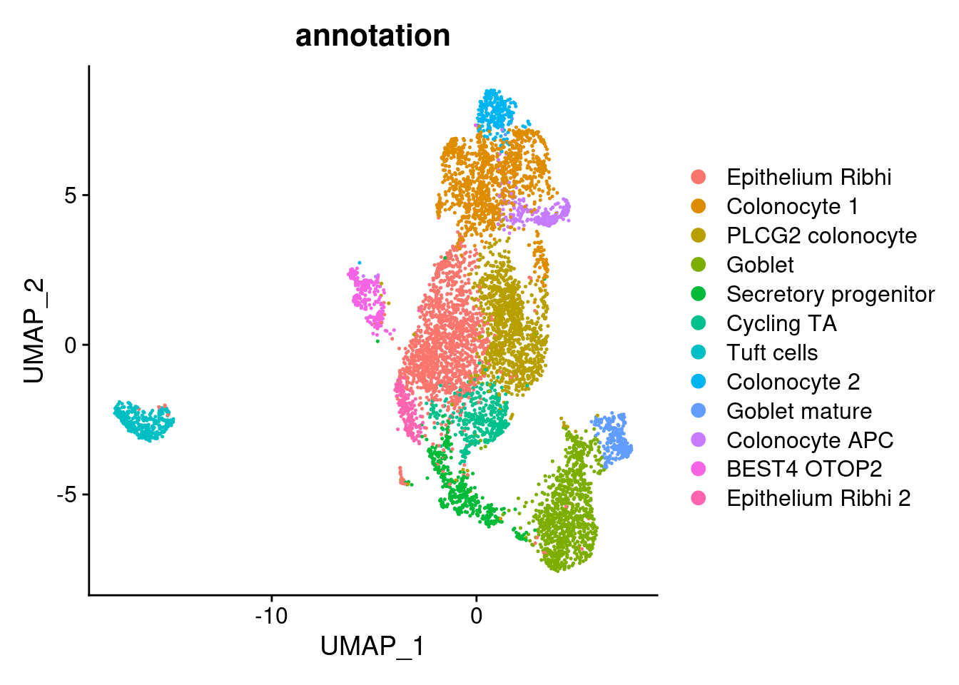
saveRDS(epi, file = 'HC/annotated/epi.RDS')Myeloid cells
MT-gene expression
Distribution of cells in scatter plot (nfeatures/percent.mt) to check where are the majority of our cells. We can see the dots colored by density using the function get_density shown in Load extra functions and sources.
myeloids <- readRDS('HC/myeloids.RDS')
meta <- myeloids@meta.data
meta$density <- get_density(meta$percent.mt, meta$nFeature_RNA, n = 100)
ggplot(meta) +
  geom_point(aes(percent.mt, nFeature_RNA, color = density), size = 0.2) +
  scale_color_viridis() + theme_classic() +
  scale_y_log10()+
  geom_vline(xintercept = 25, linetype = 2, color = 'gray')+
  theme(text = element_text( size = 12),
        axis.title = element_text( size = 12),
        legend.text = element_blank())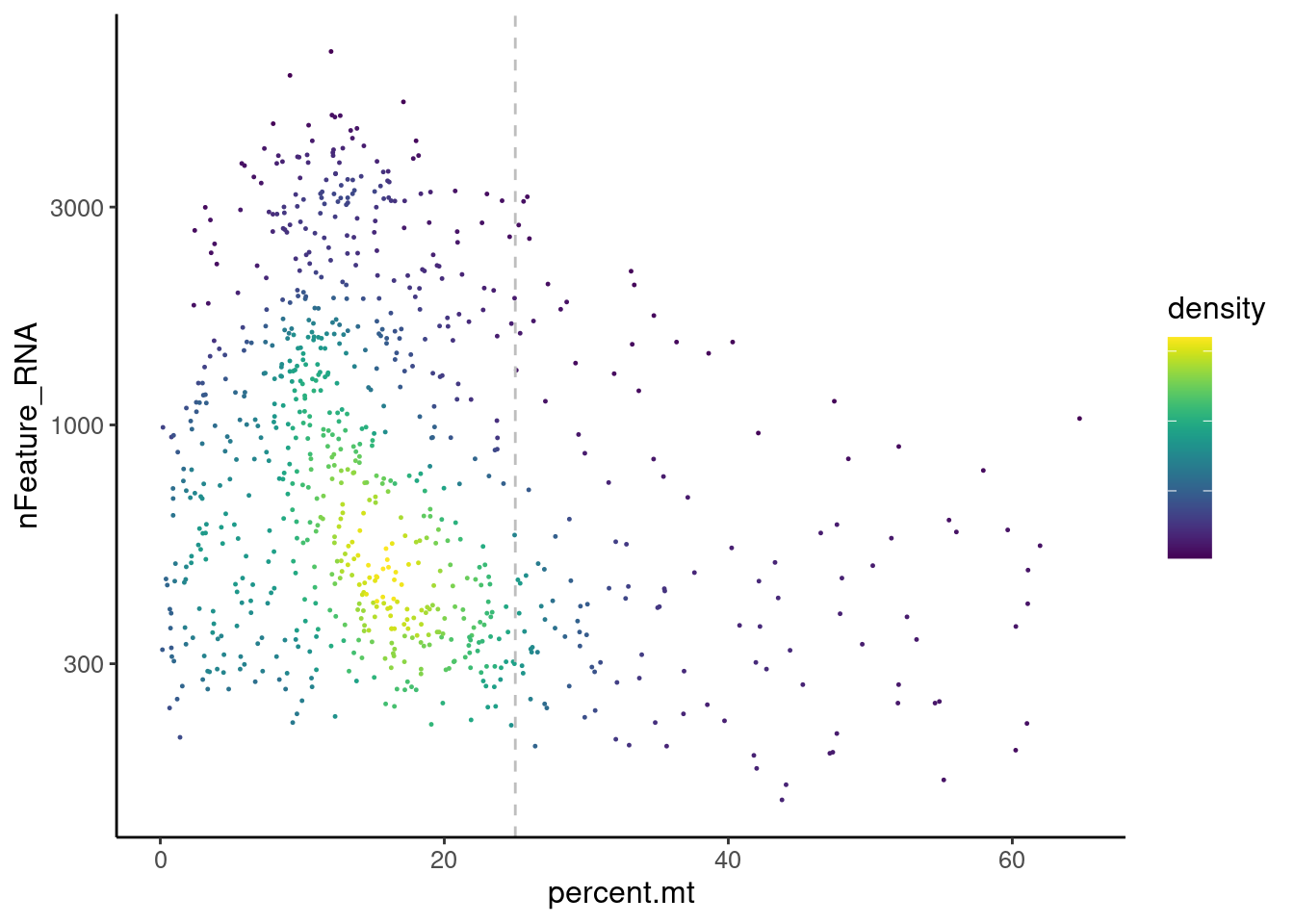
We analyzed the data using different cutoffs for the percent.mt (data not shown) and finally decided that 25% was a reasonable choice for this dataset.
myeloids <- myeloids[,myeloids$percent.mt < 25]Non-myeloid genes
Right now myeloids has 708 cells. Nevertheless, many
express genes that we know should not be expressed by myeloid cells. We
will remove those cells.
genes <-  c('CD3E','CD3D','CD3G', 'DERL3', 'MS4A1', 'CD79A','EPCAM')
for (gene in genes) {
    j <- FeaturePlot(myeloids, features = gene, order=T, reduction = 'pca') + theme_classic()
    cat("#### ", gene, "\n"); print(j); cat("\n\n")
  }
CD3E
CD3D

CD3G

DERL3

MS4A1
CD79A
EPCAM
cat("#### code removal \n")code removal
counts <- myeloids@assays$RNA@counts
p <- grep("CD3E$|CD3D$|CD3G$|MS4A1$|DERL3|CD79A$|EPCAM$",rownames(myeloids))
pp <- which(Matrix::colSums(counts[p,])>0)
xx <-setdiff(colnames(myeloids), names(pp))
myeloids <- subset(myeloids,cells = xx)
cat('\n\n')
Ig genes signal
We have observed that due to normalization, there’s high Ig gene expression in cells that did not have high counts of Ig genes. As an example:
a <- FeaturePlot(myeloids, features = 'IGHA1', slot = 'counts', order = T) + labs(title='counts') + theme_classic()
b <- FeaturePlot(myeloids, features = 'IGHA1', slot = 'data', order = T) + labs(title= 'data') + theme_classic()
wrap_plots(a,b, nrow = 1)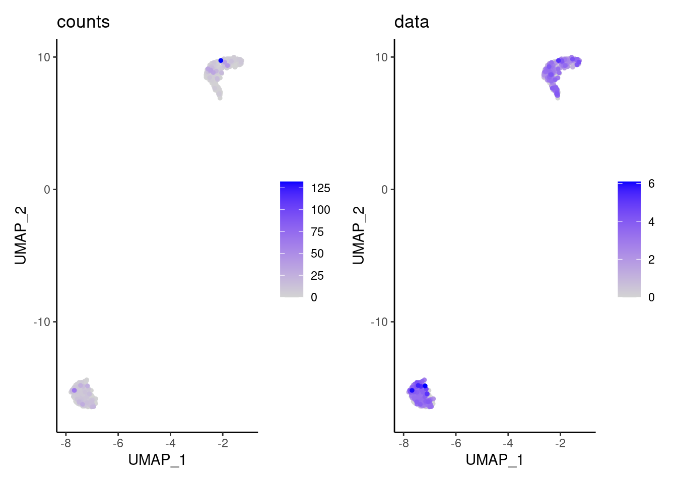
We remove the Ig genes from the dataset in all subsets except for the plasma and B cells subset.
gg <- rownames(myeloids)[c(grep("^IGH",rownames(myeloids)),
                         grep("^IGK", rownames(myeloids)),
                         grep("^IGL", rownames(myeloids)))]
genes <- setdiff(rownames(myeloids),gg)
myeloids <- subset(myeloids,features = genes)
Genes without expression
We remove the genes without expression from the dataset.
counts <- myeloids@assays$RNA@counts
pp <- which(Matrix::rowSums(counts)==0)
xx <-setdiff(rownames(myeloids), names(pp))
myeloids <- subset(myeloids, features = xx)
Dimension reduction
We tried different values of PC for the UMAP generation and Louvain clusterization. Finally, we considered 18 PCs for the analysis.
myeloids <- seurat_to_pca(myeloids)
## [1] "NORMALIZATION"
## [1] "VARIABLE FEATURES"
## [1] "SCALE DATA"
## [1] "RUN PCA"

a <- ElbowPlot(myeloids, ndims = 100) +
  geom_vline(xintercept = 18, colour="#BB0000", linetype = 2)+
  labs(title = paste0('Elbowplot')) + theme_classic()

myeloids <- FindNeighbors(myeloids, dims = 1:18)
myeloids <-RunUMAP(myeloids, dims=1:18)
b <- DimPlot(myeloids, group.by = 'sample_name') +
  labs(title = '18 PCS') +
  theme_classic() +
  theme(legend.position = 'bottom')

(a+b) / guide_area() +
  plot_layout(heights = c(0.7,0.3),guides = 'collect')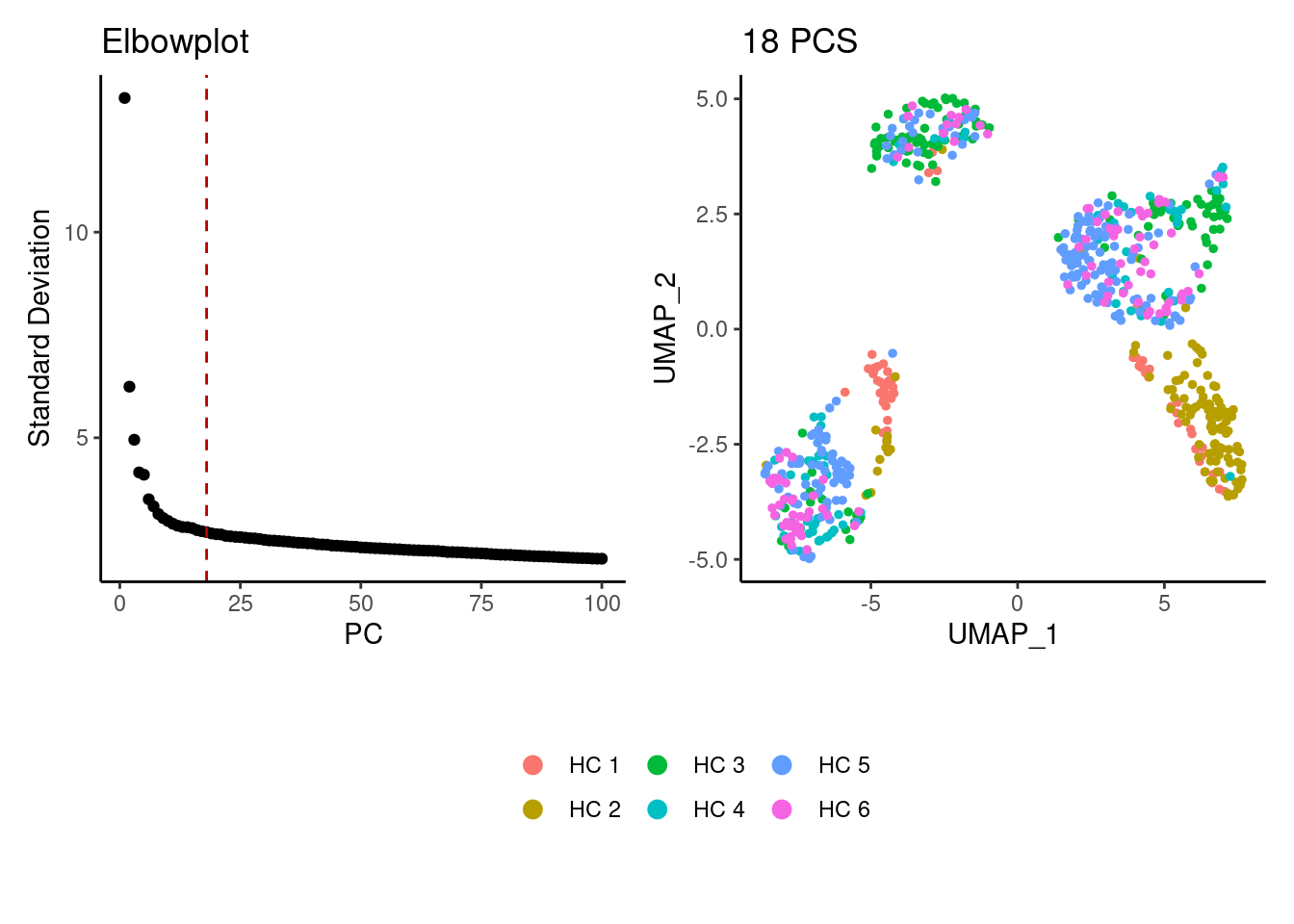
Harmony correction
myeloids <- RunHarmony(myeloids, group.by = 'sample_name', dims.use = 1:18)
a <- ElbowPlot(myeloids, ndims = 100, reduction = 'harmony') +
  geom_vline(xintercept = 19, linetype = 2)
myeloids<- FindNeighbors(myeloids, reduction = "harmony", dims = 1:19)
myeloids<-RunUMAP(myeloids, dims=1:19, reduction= "harmony")

b <- DimPlot(myeloids, group.by = 'sample_name') + theme_classic() +
  theme(legend.position = 'bottom')

(a+b) / guide_area() +
  plot_layout(heights = c(0.7,0.3),guides = 'collect')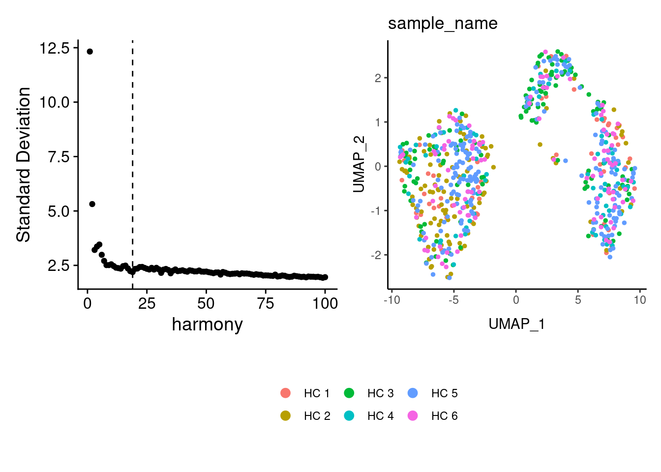
Louvain Clusterization
dir.create('HC/Myeloids')
path <- getwd()
myeloids <- resolutions(myeloids,
                   workingdir = path,
                   title = 'HC/Myeloids/Markers_Myeloids_')
saveRDS(myeloids, file = 'HC/Myeloids/myeloids_filtered.RDS')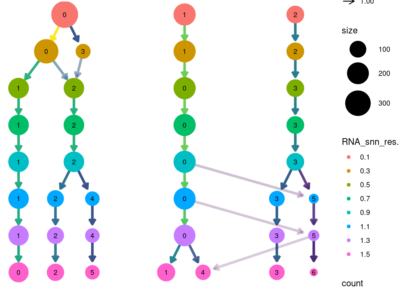
Annotation
myeloids$annotation <- plyr::mapvalues(x = myeloids$RNA_snn_res.0.5,
                                       from = 0:3,
                                       to = c("M2",
                                              "Macrophage Ribhi",
                                              "Mast",
                                              "M0"))

DimPlot(myeloids, group.by = 'annotation') 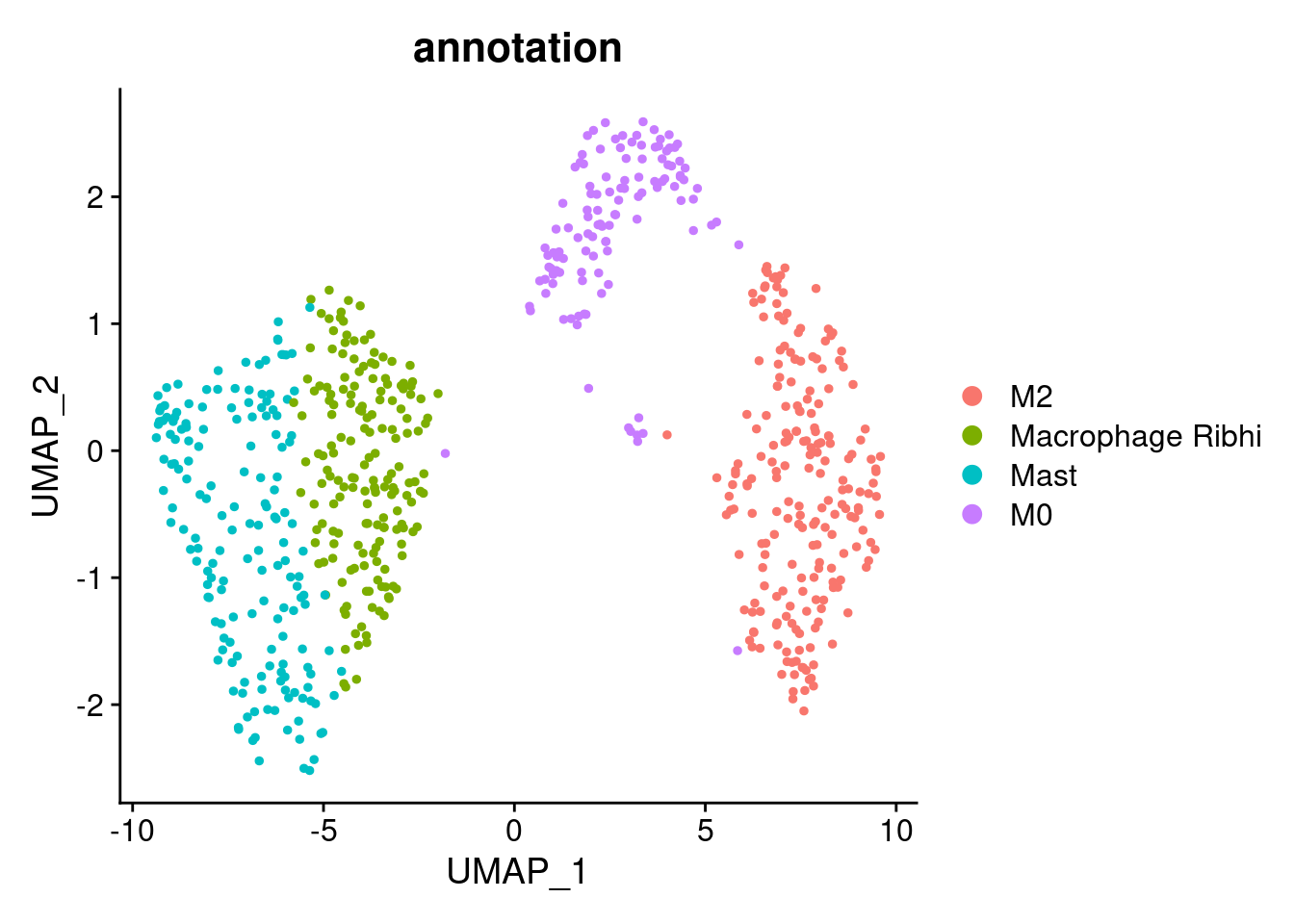
saveRDS(myeloids, file = 'HC/annotated/myeloids.RDS')Stromal cells
MT-gene expression
Distribution of cells in scatter plot (nfeatures/percent.mt) to check where are the majority of our cells. We can see the dots colored by density using the function get_density shown in Load extra functions and sources.
stroma <- readRDS('HC/stroma.RDS')
meta <- stroma@meta.data
meta$density <- get_density(meta$percent.mt, meta$nFeature_RNA, n = 100)
ggplot(meta) +
geom_point(aes(percent.mt, nFeature_RNA, color = density), size = 0.2) +
scale_color_viridis() + theme_classic() +
scale_y_log10()+
geom_vline(xintercept = 25, linetype = 2, color = 'gray')+
theme(text = element_text( size = 12),
axis.title = element_text( size = 12),
legend.text = element_blank())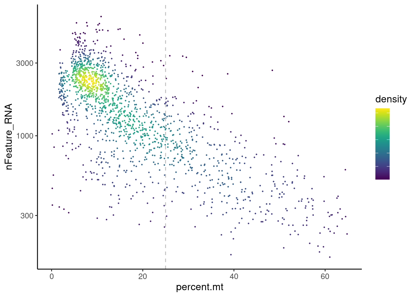 We analyzed the data using different cutoffs for the percent.mt (data
not shown) and finally decided that 25% was a reasonable choice for our
dataset.
We analyzed the data using different cutoffs for the percent.mt (data
not shown) and finally decided that 25% was a reasonable choice for our
dataset.
stroma <- stroma[,stroma$percent.mt < 25]Non-stromal genes
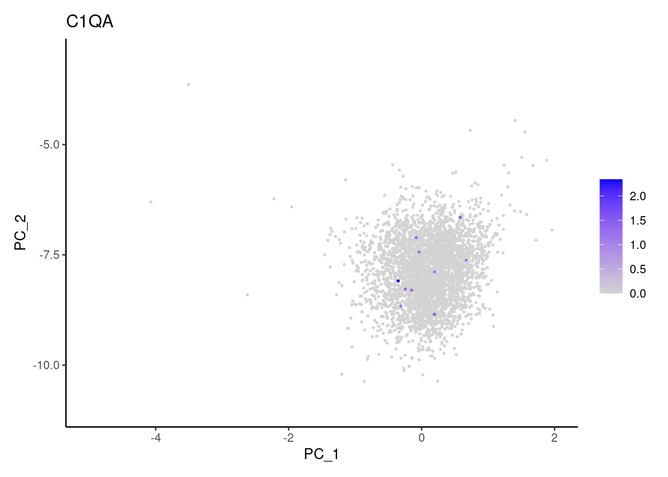
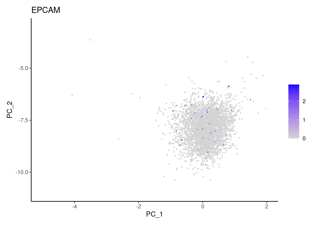
Right now stroma has 1231 cells. Nevertheless, many cells express genes that we know should not be expressed by stromal cells. We will remove those cells.
genes <-  c('CD3E','CD3D','CD3G', 'C1QA',
            'DERL3', 'MS4A1', 'C1QA', 'EPCAM')
for (gene in genes) {
    j <- FeaturePlot(stroma, features = gene, order=T, reduction = 'pca') + theme_classic()
    cat("#### ", gene, "\n"); print(j); cat("\n\n")
  }
CD3E

CD3D

CD3G

C1QA

DERL3
MS4A1
C1QA
EPCAM
cat("#### code removal \n")code removal
counts <- stroma@assays$RNA@counts
p <- grep("CD3E$|CD3D$|CD3G$|MS4A1$|DERL3|^C1QA$|^EPCAM$",rownames(stroma))
pp <- which(Matrix::colSums(counts[p,])>0)
xx <-setdiff(colnames(stroma), names(pp))
stroma <- subset(stroma,cells = xx)
cat('\n\n')
Ig genes signal
We have observed that due to normalization, there’s high Ig gene expression in cells that did not have high counts of Ig genes. As an example:
a <- FeaturePlot(stroma, features = 'IGHA1', slot = 'counts', order=T) + labs(title='counts') + theme_classic()
b <- FeaturePlot(stroma, features = 'IGHA1', slot = 'data', order=T) + labs(title= 'data') + theme_classic()
wrap_plots(a,b, nrow = 1)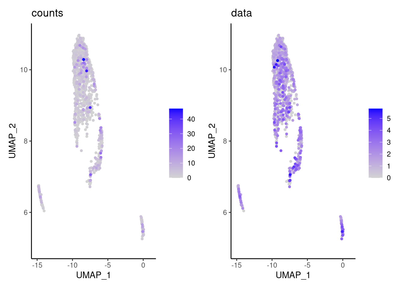
We remove the Ig genes from the dataset in all subsets except for the plasma and B cells subset.
gg <- rownames(stroma)[c(grep("^IGH",rownames(stroma)),
                         grep("^IGK", rownames(stroma)),
                         grep("^IGL", rownames(stroma)))]
genes <- setdiff(rownames(stroma),gg)
stroma <- subset(stroma,features = genes)
Genes wo expression
We remove the genes without expression from the dataset.
counts <- stroma@assays$RNA@counts
pp <- which(Matrix::rowSums(counts)==0)
xx <-setdiff(rownames(stroma), names(pp))
stroma <- subset(stroma, features = xx)
Dimension reduction
stroma <- seurat_to_pca(stroma)
## [1] "NORMALIZATION"
## [1] "VARIABLE FEATURES"
## [1] "SCALE DATA"
## [1] "RUN PCA"

a <- ElbowPlot(stroma, ndims = 100) +
  geom_vline(xintercept = 25, colour="#BB0000", linetype = 2)+
  labs(title = paste0('Elbowplot')) + theme_classic()

stroma<- FindNeighbors(stroma, dims = 1:25)
stroma<-RunUMAP(stroma, dims=1:25)
b <- DimPlot(stroma, group.by = 'sample_name') +
  labs(title = '25 PCS') +
  theme_classic() +
  theme(legend.position = 'bottom')

(a+b) / guide_area() +
  plot_layout(heights = c(0.7,0.3),guides = 'collect')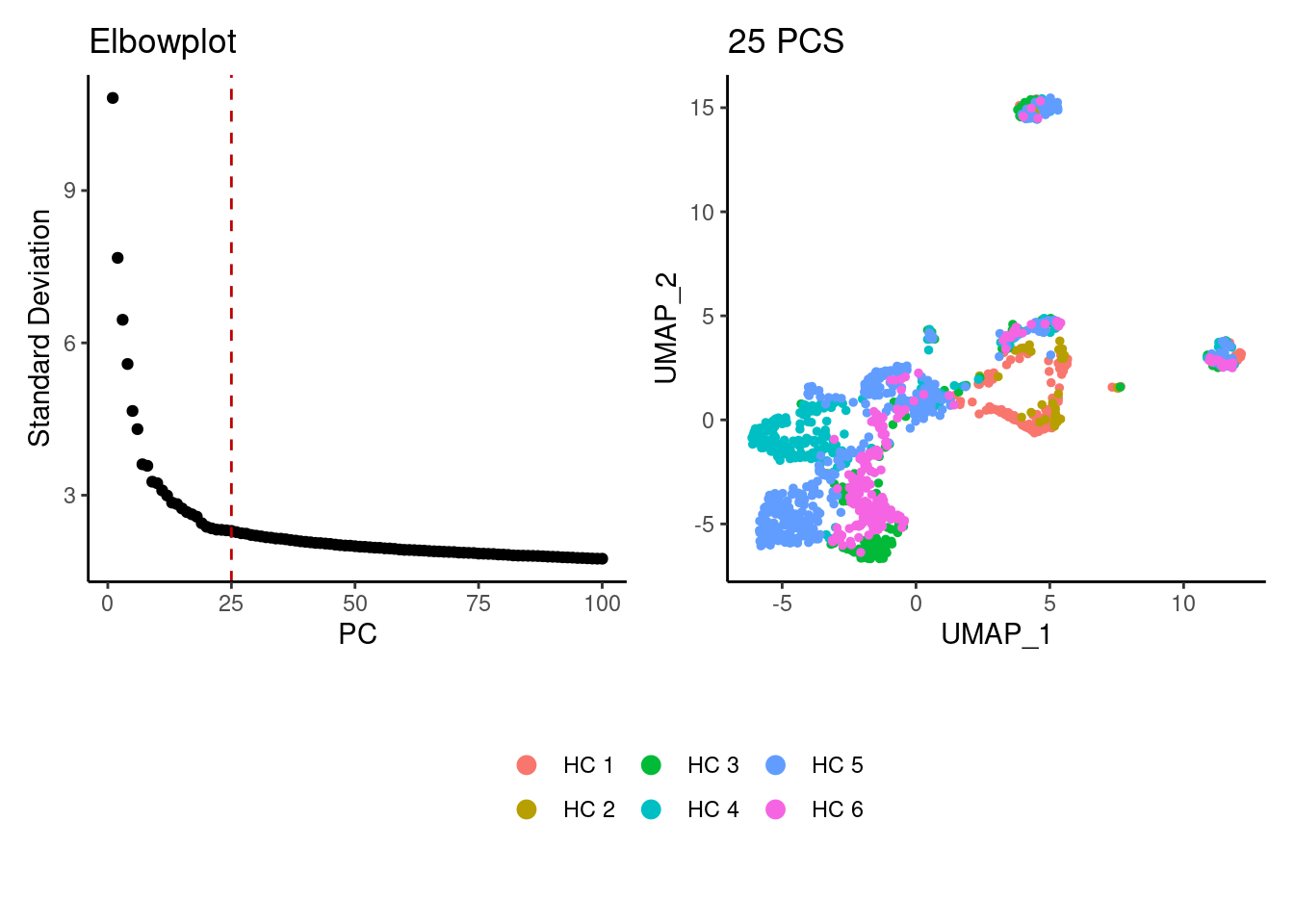
Harmony correction
stroma <- RunHarmony(stroma, group.by = 'sample_name', dims.use = 1:25)

a <- ElbowPlot(stroma, reduction = 'harmony', ndims = 100) +
  geom_vline(xintercept = 27, colour="#BB0000", linetype = 2)+
  labs(title = paste0('Elbowplot'))+ theme_classic()

stroma<- FindNeighbors(stroma, reduction = "harmony", dims = 1:27)
stroma<-RunUMAP(stroma, dims=1:27, reduction= "harmony")

b <- DimPlot(stroma, group.by = 'sample_name', pt.size = 0.1) +
  theme_classic() +
  theme(legend.position = 'bottom')

(a+b) / guide_area() +
  plot_layout(heights = c(0.7,0.3),guides = 'collect')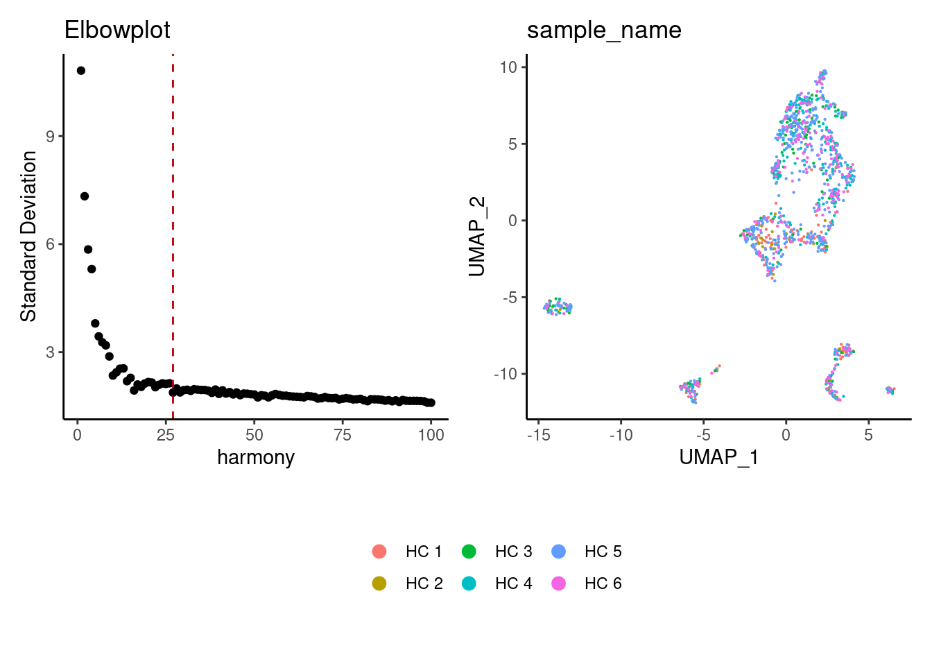
Louvain Clusterization
dir.create('HC/Stroma')
path <- getwd()
stroma <- resolutions(stroma,
                   workingdir = path,
                   title = 'HC/Stroma/Markers_Stroma_')
saveRDS(stroma, file = 'HC/Stroma/stroma_filtered.RDS')
clustree(stroma, prefix = 'RNA_snn_res.')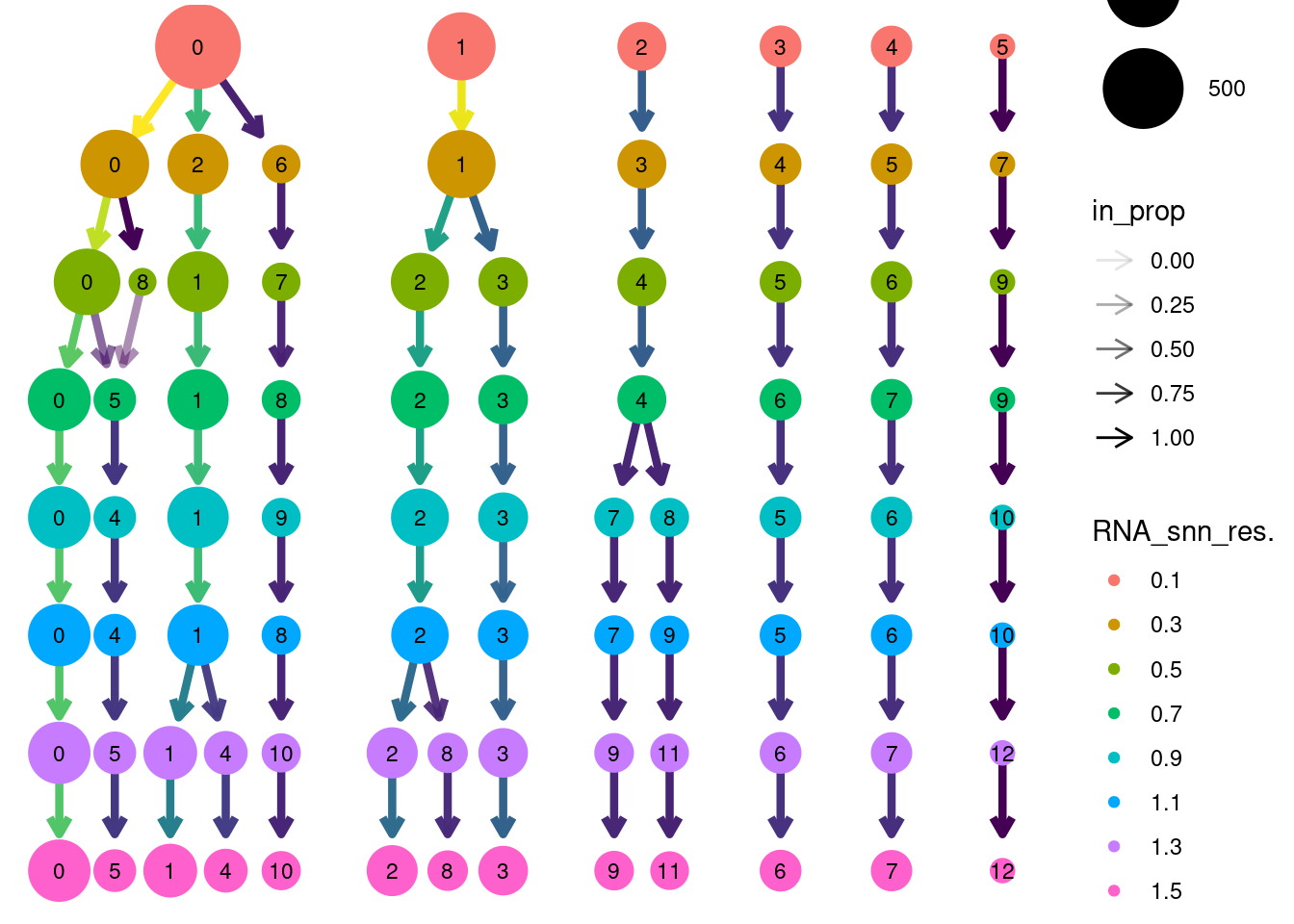
Annotation
stroma$annotation <- plyr::mapvalues(x = stroma$RNA_snn_res.0.9,
                                       from = 0:10,
                                       to = c("S1",
                                              "IER fibroblasts",
                                              "S1 Ribhi",
                                              "MT fibroblasts",
                                              "Fibroblasts Ribhi",
                                              "Endothelium",
                                              "Glia",
                                              "S2a",
                                              "S2b",
                                              "S3",
                                              "Myofibroblasts"))

DimPlot(stroma, group.by = 'annotation') 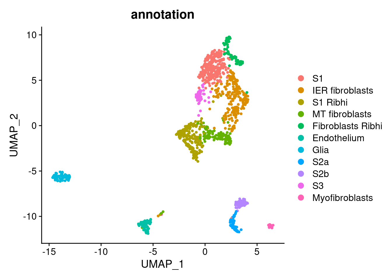
saveRDS(stroma, file = 'HC/annotated/stroma.RDS')SessionInfo
sessionInfo()
## R version 4.1.2 (2021-11-01)
## Platform: x86_64-pc-linux-gnu (64-bit)
## Running under: Ubuntu 20.04.5 LTS
##
## Matrix products: default
## BLAS:   /usr/lib/x86_64-linux-gnu/blas/libblas.so.3.9.0
## LAPACK: /opt/R/4.1.2/lib/R/lib/libRlapack.so
##
## locale:
##  [1] LC_CTYPE=C.UTF-8       LC_NUMERIC=C           LC_TIME=C.UTF-8        LC_COLLATE=C.UTF-8
##  [5] LC_MONETARY=C.UTF-8    LC_MESSAGES=C          LC_PAPER=C.UTF-8       LC_NAME=C
##  [9] LC_ADDRESS=C           LC_TELEPHONE=C         LC_MEASUREMENT=C.UTF-8 LC_IDENTIFICATION=C
##
## attached base packages:
## [1] stats4    stats     graphics  grDevices utils     datasets  methods   base
##
## other attached packages:
##  [1] harmony_0.1.0               Rcpp_1.0.9                  rmarkdown_2.18              pandoc_0.1.0
##  [5] readxl_1.3.1                magick_2.7.3                data.table_1.14.2           BiocParallel_1.28.3
##  [9] RColorBrewer_1.1-3          ggrepel_0.9.1               ggrastr_1.0.1               usethis_2.1.5
## [13] clustree_0.4.4              ggraph_2.0.5                readr_2.1.2                 dplyr_1.0.10
## [17] cowplot_1.1.1               reshape_0.8.8               formulaic_0.0.8             patchwork_1.1.2
## [21] MASS_7.3-55                 viridis_0.6.2               viridisLite_0.4.1           scDblFinder_1.8.0
## [25] scran_1.22.1                scater_1.22.0               scuttle_1.4.0               celda_1.10.0
## [29] beepr_1.3                   DropletUtils_1.14.2         SingleCellExperiment_1.16.0 SummarizedExperiment_1.24.0
## [33] Biobase_2.54.0              GenomicRanges_1.46.1        GenomeInfoDb_1.30.1         IRanges_2.28.0
## [37] S4Vectors_0.32.4            BiocGenerics_0.40.0         MatrixGenerics_1.6.0        matrixStats_0.62.0
## [41] ggplot2_3.3.6               plyr_1.8.7                  sp_1.5-0                    SeuratObject_4.1.1
## [45] Seurat_4.1.0.9007
##
## loaded via a namespace (and not attached):
##   [1] rsvd_1.0.5                 ica_1.0-3                  corpcor_1.6.10             assertive.properties_0.0-4
##   [5] foreach_1.5.2              lmtest_0.9-40              rprojroot_2.0.3            crayon_1.5.2
##   [9] spatstat.core_2.4-4        rhdf5filters_1.6.0         backports_1.4.1            nlme_3.1-155
##  [13] rlang_1.0.6                XVector_0.34.0             ROCR_1.0-11                irlba_2.3.5
##  [17] SparseM_1.81               limma_3.50.3               xgboost_1.5.0.2            rjson_0.2.21
##  [21] bit64_4.0.5                glue_1.6.2                 sctransform_0.3.4          parallel_4.1.2
##  [25] vipor_0.4.5                spatstat.sparse_2.1-1      AnnotationDbi_1.56.2       spatstat.geom_2.4-0
##  [29] tidyselect_1.1.2           fitdistrplus_1.1-8         tidyr_1.2.1                assertive.types_0.0-3
##  [33] zoo_1.8-10                 org.Mm.eg.db_3.14.0        xtable_1.8-4               magrittr_2.0.3
##  [37] evaluate_0.18              cli_3.4.0                  zlibbioc_1.40.0            rstudioapi_0.13
##  [41] miniUI_0.1.1.1             bslib_0.4.1                rpart_4.1.16               RcppEigen_0.3.3.9.2
##  [45] shiny_1.7.3                BiocSingular_1.10.0        xfun_0.34                  clue_0.3-60
##  [49] cluster_2.1.2              tidygraph_1.2.1            KEGGREST_1.34.0            tibble_3.1.8
##  [53] listenv_0.8.0              Biostrings_2.62.0          png_0.1-7                  future_1.28.0
##  [57] withr_2.5.0                bitops_1.0-7               ggforce_0.3.3              cellranger_1.1.0
##  [61] assertive.base_0.0-9       dqrng_0.3.0                pillar_1.8.1               GlobalOptions_0.1.2
##  [65] cachem_1.0.6               fs_1.5.2                   GetoptLong_1.0.5           DelayedMatrixStats_1.16.0
##  [69] vctrs_0.4.1                ellipsis_0.3.2             generics_0.1.3             tools_4.1.2
##  [73] beeswarm_0.4.0             munsell_0.5.0              tweenr_1.0.2               DelayedArray_0.20.0
##  [77] fastmap_1.1.0              compiler_4.1.2             pkgload_1.2.4              abind_1.4-5
##  [81] httpuv_1.6.6               plotly_4.10.0              rgeos_0.5-9                GenomeInfoDbData_1.2.7
##  [85] gridExtra_2.3              enrichR_3.0                edgeR_3.36.0               lattice_0.20-45
##  [89] deldir_1.0-6               utf8_1.2.2                 later_1.3.0                jsonlite_1.8.3
##  [93] multipanelfigure_2.1.2     scales_1.2.1               graph_1.72.0               ScaledMatrix_1.2.0
##  [97] pbapply_1.5-0              sparseMatrixStats_1.6.0    lazyeval_0.2.2             promises_1.2.0.1
## [101] doParallel_1.0.17          R.utils_2.12.0             goftest_1.2-3              checkmate_2.0.0
## [105] spatstat.utils_2.3-1       reticulate_1.26            textshaping_0.3.6          statmod_1.4.36
## [109] Rtsne_0.16                 uwot_0.1.14                igraph_1.3.4               HDF5Array_1.22.1
## [113] survival_3.2-13            rsconnect_0.8.25           yaml_2.3.6                 systemfonts_1.0.4
## [117] htmltools_0.5.3            memoise_2.0.1              locfit_1.5-9.6             graphlayouts_0.8.0
## [121] digest_0.6.30              assertthat_0.2.1           rappdirs_0.3.3             mime_0.12
## [125] RSQLite_2.2.17             future.apply_1.9.1         blob_1.2.3                 R.oo_1.25.0
## [129] ragg_1.2.1                 splines_4.1.2              labeling_0.4.2             Rhdf5lib_1.16.0
## [133] RCurl_1.98-1.8             assertive.numbers_0.0-2    hms_1.1.1                  rhdf5_2.38.1
## [137] colorspace_2.0-3           ggbeeswarm_0.6.0           shape_1.4.6                assertive.files_0.0-2
## [141] matchSCore2_0.1.0          nnet_7.3-17                sass_0.4.2                 RANN_2.6.1
## [145] circlize_0.4.14            audio_0.1-10               fansi_1.0.3                tzdb_0.2.0
## [149] brio_1.1.3                 parallelly_1.32.1          R6_2.5.1                   grid_4.1.2
## [153] ggridges_0.5.3             lifecycle_1.0.3            formatR_1.12               bluster_1.4.0
## [157] curl_4.3.2                 jquerylib_0.1.4            leiden_0.4.3               testthat_3.1.2
## [161] Matrix_1.4-0               desc_1.4.0                 RcppAnnoy_0.0.19           org.Hs.eg.db_3.14.0
## [165] iterators_1.0.14           stringr_1.4.1              topGO_2.46.0               htmlwidgets_1.5.4
## [169] beachmat_2.10.0            polyclip_1.10-0            purrr_0.3.4                gridGraphics_0.5-1
## [173] ComplexHeatmap_2.10.0      mgcv_1.8-38                globals_0.16.1             spatstat.random_2.2-0
## [177] progressr_0.11.0           codetools_0.2-18           GO.db_3.14.0               metapod_1.2.0
## [181] MCMCprecision_0.4.0        R.methodsS3_1.8.2          gtable_0.3.1               DBI_1.1.3
## [185] highr_0.9                  tensor_1.5                 httr_1.4.4                 KernSmooth_2.23-20
## [189] vroom_1.5.7                stringi_1.7.8              reshape2_1.4.4             farver_2.1.1
## [193] combinat_0.0-8             BiocNeighbors_1.12.0       scattermore_0.8            bit_4.0.4
## [197] spatstat.data_2.2-0        pkgconfig_2.0.3            corrplot_0.92              knitr_1.40