Data together and first quality control
Last compiled on 17 November, 2022
Data together
Load libraries
library(Seurat)
library(plyr)
library(ggplot2)
library(DropletUtils)
library(celda)
library(SingleCellExperiment)
library(scater)
library(scran)
library(scDblFinder)
library(viridis)
library(MASS)
library(patchwork)
Load extra sources
get_density <- function(x, y, ...) { # function from https://slowkow.com/notes/ggplot2-color-by-density/
  dens <- MASS::kde2d(x, y, ...)
  ix <- findInterval(x, dens$x)
  iy <- findInterval(y, dens$y)
  ii <- cbind(ix, iy)
  return(dens$z[ii])
}

fancy_scientific <- function(l) { # function from https://stackoverflow.com/a/24241954
     # turn in to character string in scientific notation
     l <- format(l, scientific = TRUE)
     # quote the part before the exponent to keep all the digits
     l <- gsub("^(.*)e", "'\\1'e", l)
     # turn the 'e+' into plotmath format
     l <- gsub("e", "%*%10^", l)
     # return this as an expression
     parse(text=l)
}

setwd("~/000_GitHub/ibd-bcn_single_cell")
source('source/functions_scrnaseq.R')
source('source/colors.R')
Sample Metadata
Metadata of the samples inside the code.
metadata <- data.frame(
  stringsAsFactors = FALSE,
  sample = c("SC_002",
             "SC_004","SC_005","SC_008","SC_010","SC_011",
             "SC_013","SC_014","SC_015","SC_016","SC_017",
             "SC_018","SC_019","SC_021","TOF001W0","TOF002W0",
             "TOF005W0","TOF010W0"),
  sample_name = factor(c("HC 1", "CD 1", "CD 2", "UC 1", "UC 2", "HC 2",
                         "CD 3", "CD 4", "HC 3", "HC 4", "HC 5", "HC 6",
                         "CD 5", "CD 6", "UC 3", "UC 4", "UC 5", "UC 6"),
                       levels = c("HC 1", "HC 2", "HC 3", "HC 4",
                                  "HC 5", "HC 6", "CD 1", "CD 2",
                                  "CD 3", "CD 4", "CD 5", "CD 6",
                                  "UC 1", "UC 2", "UC 3", "UC 4",
                                  "UC 5", "UC 6")),
  Health = factor(c("HC", "CDa", "CDa","UCa","UCa","HC","CDa","CDa",
                    "HC","HC","HC","HC","CDa","CDa","UCa","UCa","UCa",
                    "UCa"), levels = c("HC", "CDa", "UCa")),
  Health_2 = factor(c("HC","IBD",
                      "IBD","IBD","IBD","HC","IBD","IBD","HC","HC",
                      "HC","HC","IBD","IBD","IBD","IBD","IBD",
                      "IBD"), levels = c("HC", "IBD"))
)
Merge data (Seurat)
This code consists of a loop joining the data. First loads the
sample, adds the sample’s metadata m4, and calculates the
doublets and MT%. Puts each sample in an empty list
list_data, and after the loop, merges the samples of the
list using Seurat’s function merge into the new
seudata object.
setwd('~/data_Albas/DATA/') # Dir where we have a folder per sample, with the 3 files from
# outs/filtered_feature_bc_matrix from cellranger output.

list_files <- list.files() # folder names
list_data <- list() # empty list

for(i in list_files){
  # read the files
  sce2 <- Read10X(i)

  # feature filtering
  keep_feature <- rowSums(sce2 > 0) > 0
  sce2 <- sce2[keep_feature, ]

  # doublet finding
  sce2 <- scDblFinder(sce2, verbose=FALSE)

  # metadata of sample
  m4 <- data.frame('sample' = rep(i, ncol(sce2)),
                   'doublet' = sce2$scDblFinder.class,
                   'Health' = rep(metadata[metadata$sample == i, 'Health'][1], ncol(sce2)),
                   'sample_name' = rep(metadata[metadata$sample == i, 'sample_name'][1], ncol(sce2)),
                   'Health_2' = rep(metadata[metadata$sample == i, 'Health_2'][1], ncol(sce2)))

  # identify sample per colname
  colnames(sce2) <- paste(i, colnames(sce2), sep='_')
  rownames(m4) <- colnames(sce2)

  # seurat of the sample
  data <- CreateSeuratObject(
    counts(sce2),
    min.features = 100,
    project = i,
    assay = "RNA",
    meta.data = m4
  )

  # calcules the percent.mt per sample
  data[["percent.mt"]] <- PercentageFeatureSet(object = data, pattern = "^MT-")

  # add each sample into the empty list
  list_data[[i]] <- data
}

seudata <- list_data[[1]]
for(i in 2:length(list_files)){
  seudata <- merge(seudata, list_data[[i]])
}
Data exploration and QC
Violin Plots
Let’s check the MT% per cell and the number of genes per cell in each sample.
VlnPlot(seudata, features = c('percent.mt', 'nFeature_RNA'),
        group.by = 'sample_name', pt.size = 0) &
  theme(text = element_text(family = 'Helvetica', size = 10),
        axis.text.x = element_text(angle = 90, vjust = 0.5,
                                   family = 'Helvetica', size = 10),
        axis.title.x = element_blank(),
        axis.text.y = element_text(family = 'Helvetica', size = 10)) &
  scale_fill_manual(values = c('#71ad96','#5fb392','#71bda0',
                               '#77c9a9','#82ceb1','#9debcc',
                               '#5d5c84','#525174','#6f6f9b',
                               '#7b7ba3','#8787ab','#9f9fbc',
                               '#bc9338','#c79d43','#cba552',
                               '#d0ad62','#d5b572','#dec691'))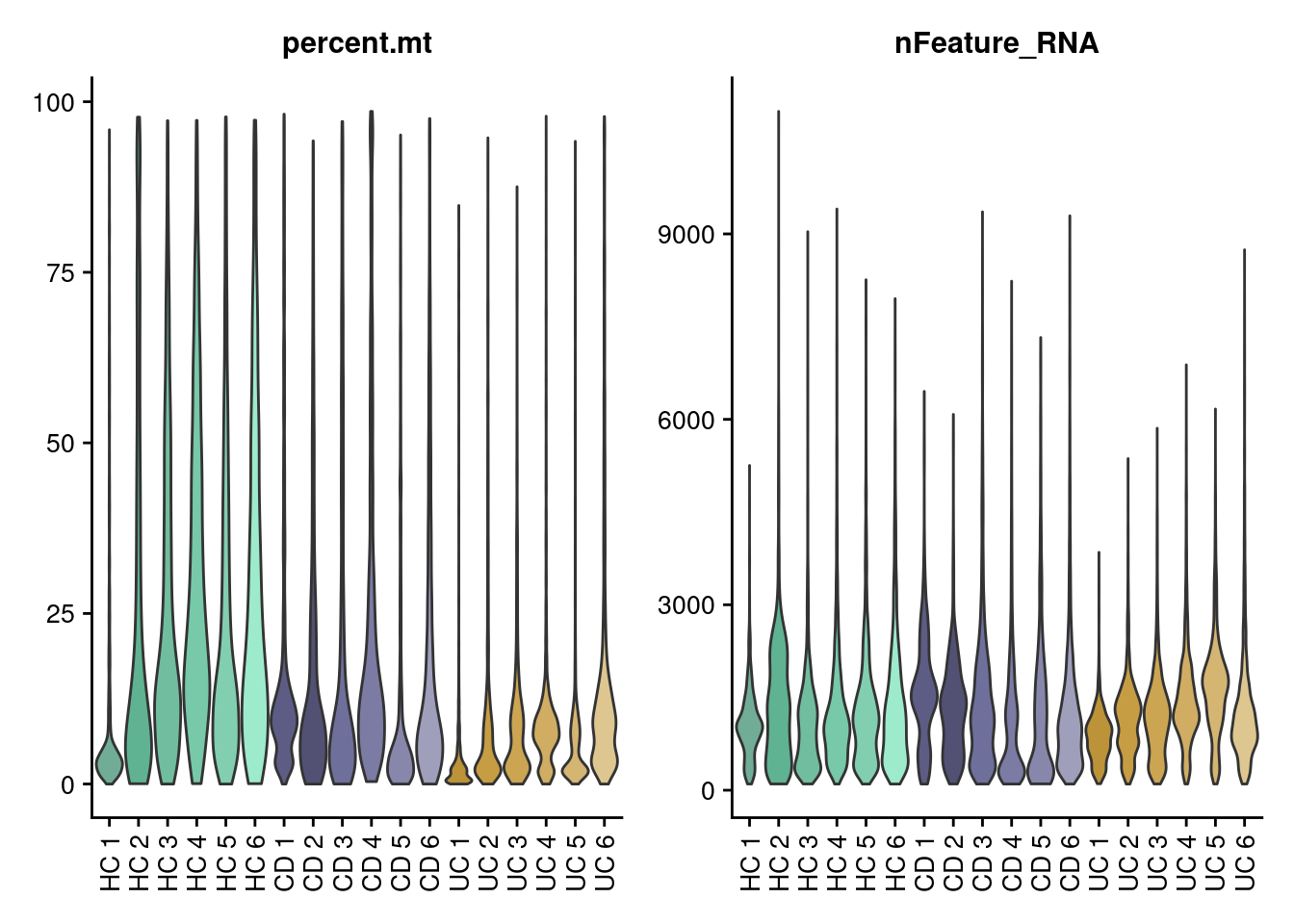
Scatter plot
Let’s check the distribution of the cells considering the total number of counts and the total number of genes per cell. First plot is colored by doublet. Second plot is colored by sample_name.
Doublets
meta <- seudata@meta.data
meta <- meta[order(meta$doublet, decreasing = T),]
ggplot(meta) +
  geom_point(aes(nCount_RNA, nFeature_RNA, color = doublet), size=0.2) +
  theme_classic() +
  scale_color_manual(values = c('doublet' = '#F6AE2DCC',
                                'singlet' = '#86BBD860'))+
  theme(plot.title = element_text(size = 25))+
  scale_x_continuous(labels=fancy_scientific) +
  theme(text = element_text(family = 'Helvetica', size = 10),
        axis.text.x = element_text(family = 'Helvetica', size = 10),
        axis.text.y = element_text(family = 'Helvetica', size = 10),
        legend.key.size = unit(5,"bigpts"), legend.title = element_blank())+
  guides(color = guide_legend(override.aes = list(size = 1.2)))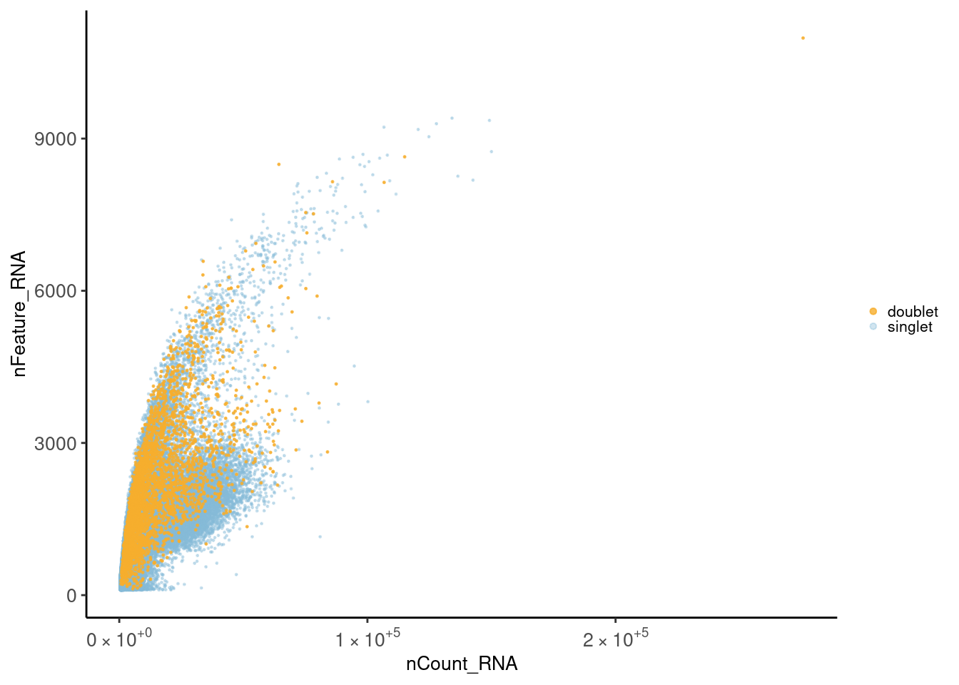
Sample
meta_dot <-  seudata@meta.data[sample(1:nrow(seudata@meta.data)), ]
sum(is.na(meta_dot$sample_name))
## [1] 0ggplot(meta_dot) +
geom_point(aes(x = nCount_RNA, y = nFeature_RNA, color = sample_name),
size = 0.2) +
theme_classic()+
scale_x_continuous(labels=fancy_scientific) +
scale_y_continuous(labels=fancy_scientific) +
scale_color_manual(values = c('#71ad9680','#5fb39280','#71bda080',
'#77c9a980','#82ceb180','#9debcc80',
'#5d5c8480','#52517480','#6f6f9b80',
'#7b7ba380','#8787ab80','#9f9fbc80',
'#bc933880','#c79d4380','#cba55280',
'#d0ad6280','#d5b57280','#dec69180'))+
guides(color = guide_legend(override.aes = list(size = 1.2), ncol=3))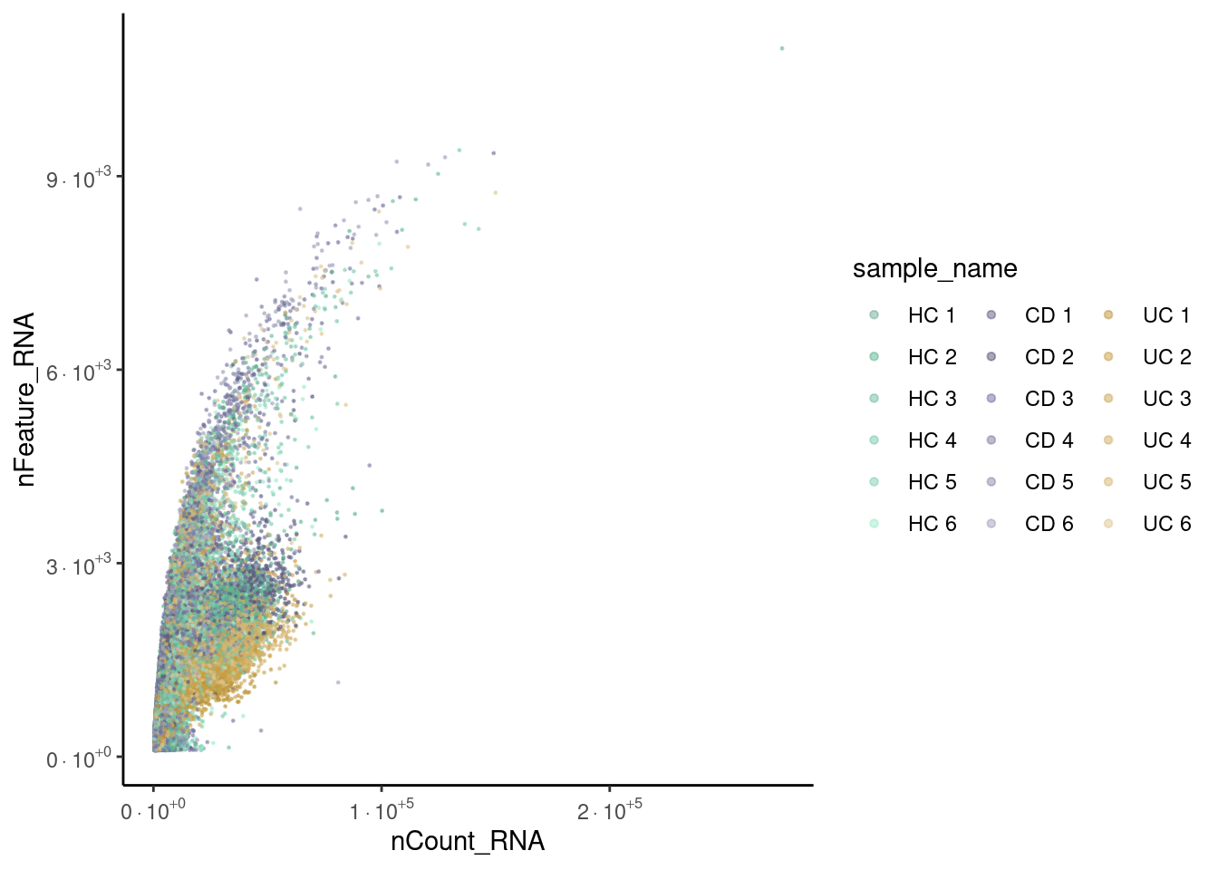
Filtering
We first filter out the cells that are considered doublets and let’s recheck the distribution of the cells after filtering.
Number of cells/sample
Tables showing the number of cells classified as singlet and doublet.
The table shows the global numbers. The barplot shows singlets/doublets
per sample. In the code, we filter out the cells classified as doublet
into a new object seudataf.
ta <- as.data.frame(table(seudata$doublet))
colnames(ta) <- c('category', 'n_cells')
knitr::kable(ta)| category | n_cells |
|---|---|
| doublet | 3333 |
| singlet | 54221 |
ta2 <- as.data.frame(table(seudata$sample_name, seudata$doublet))
colnames(ta2) <- c('sample','doublet','n_cells')
ta2$sample <- factor(ta2$sample, levels = c("HC 1", "HC 2", "HC 3", "HC 4",
"HC 5", "HC 6", "CD 1", "CD 2",
"CD 3", "CD 4", "CD 5", "CD 6",
"UC 1", "UC 2", "UC 3", "UC 4",
"UC 5", "UC 6"))
ggplot(data=ta2, aes(x=sample, y=n_cells, fill=doublet)) +
geom_bar(stat="identity", position=position_dodge())+
geom_text(aes(label=n_cells), vjust=1.6, color="black",
position = position_dodge(0.9), size=2.5)+
scale_fill_manual(values = c('doublet' = '#F6AE2DCC',
'singlet' = '#86BBD860'))+
labs(y = 'number of cells') +
theme_classic()+
theme(axis.text.x = element_text(angle=90, vjust=0.5),
legend.title = element_blank(),
axis.title.x= element_blank())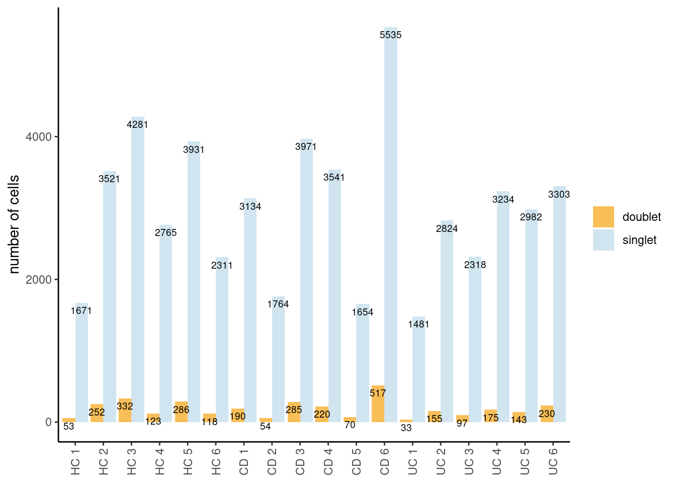
seudataf <- seudata[,seudata$doublet == 'singlet']Distribution after doublet filtering
nCount/nFeatures
Distribution of cells in the scatter plot (ncount/nfeatures) without the doublets.
meta_dot <- seudataf@meta.data[sample(1:nrow(seudataf@meta.data)), ]
ggplot(meta_dot) +
  geom_point(aes(x = nCount_RNA, y = nFeature_RNA, color = sample_name),
             size = 0.2) +
  theme_classic()+
  scale_x_continuous(labels=fancy_scientific) +
  scale_y_continuous(labels=fancy_scientific) +
  scale_color_manual(values = c('#71ad9680','#5fb39280','#71bda080',
                                '#77c9a980','#82ceb180','#9debcc80',
                                '#5d5c8480','#52517480','#6f6f9b80',
                                '#7b7ba380','#8787ab80','#9f9fbc80',
                                '#bc933880','#c79d4380','#cba55280',
                                '#d0ad6280','#d5b57280','#dec69180'))+
  guides(color = guide_legend(override.aes = list(size = 1.2), ncol=3))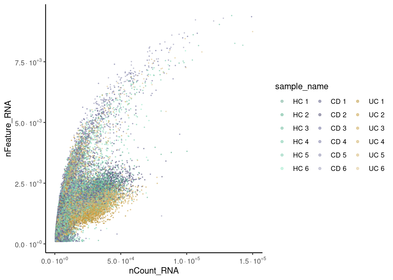
DERL3 expression
Plasma cells have more counts than other cells with the same number of features.
seudataf2 <- seudataf
meta_dot2 <- FetchData(seudataf2, vars = c('nCount_RNA', 'nFeature_RNA', 'DERL3'))
meta_dot2$DERL3_scaled <- scale(meta_dot2$DERL3)[,1]
meta_dot2 <- meta_dot2[order(meta_dot2$DERL3_scaled),]
ggplot(meta_dot2) +
  geom_point(aes(x = nCount_RNA, y = nFeature_RNA, color = DERL3_scaled),
             size = 0.2) +
  theme_classic()+
  scale_color_distiller("scaled/nDERL3",
                        limits = c(min(meta_dot2$DERL3_scaled, na.rm = T),
                                   max(meta_dot2$DERL3_scaled, na.rm=T)),
                        na.value = "white", palette = "YlOrRd", direction = 1) +
  scale_x_continuous(labels=fancy_scientific) +
scale_y_continuous(labels=fancy_scientific) 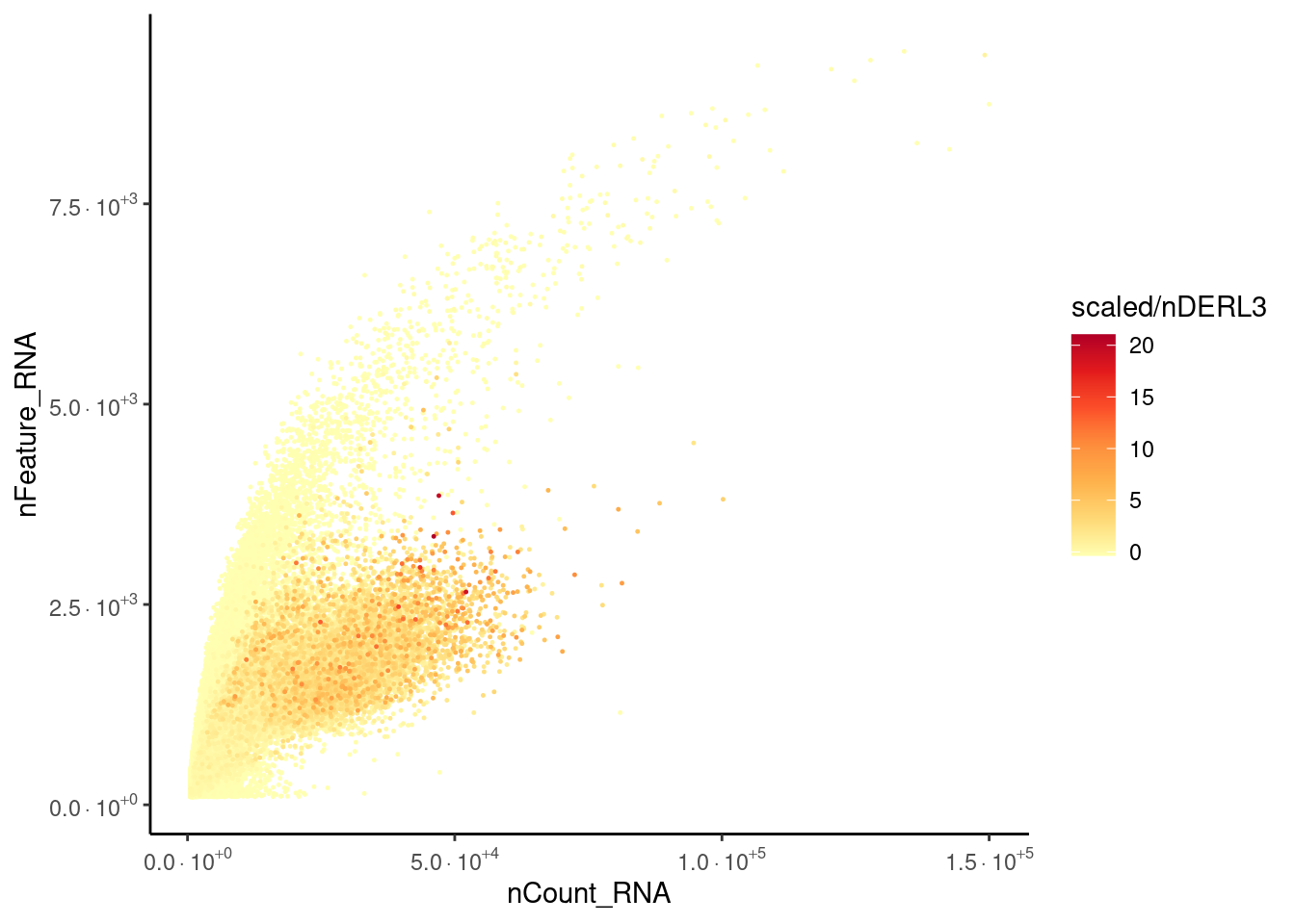
rm(seudataf2, meta_dot2)MT% filtering after doublet filtering
Distribution of cells in scatter plot (nfeatures/percent.mt) to check where are the majority of our cells. We can see the dots colored by density using the function get_density shown in [Load extra functions and sources].
All cells
meta <- seudataf@meta.data
meta$density <- get_density(meta$percent.mt, meta$nFeature_RNA, n = 100)
ggplot(meta) +
  geom_point(aes(percent.mt, nFeature_RNA, color = density), size = 0.2) +
  scale_color_viridis() + theme_classic() +
  theme(text = element_text( size = 12),
        axis.title = element_text( size = 12),
        legend.text = element_blank())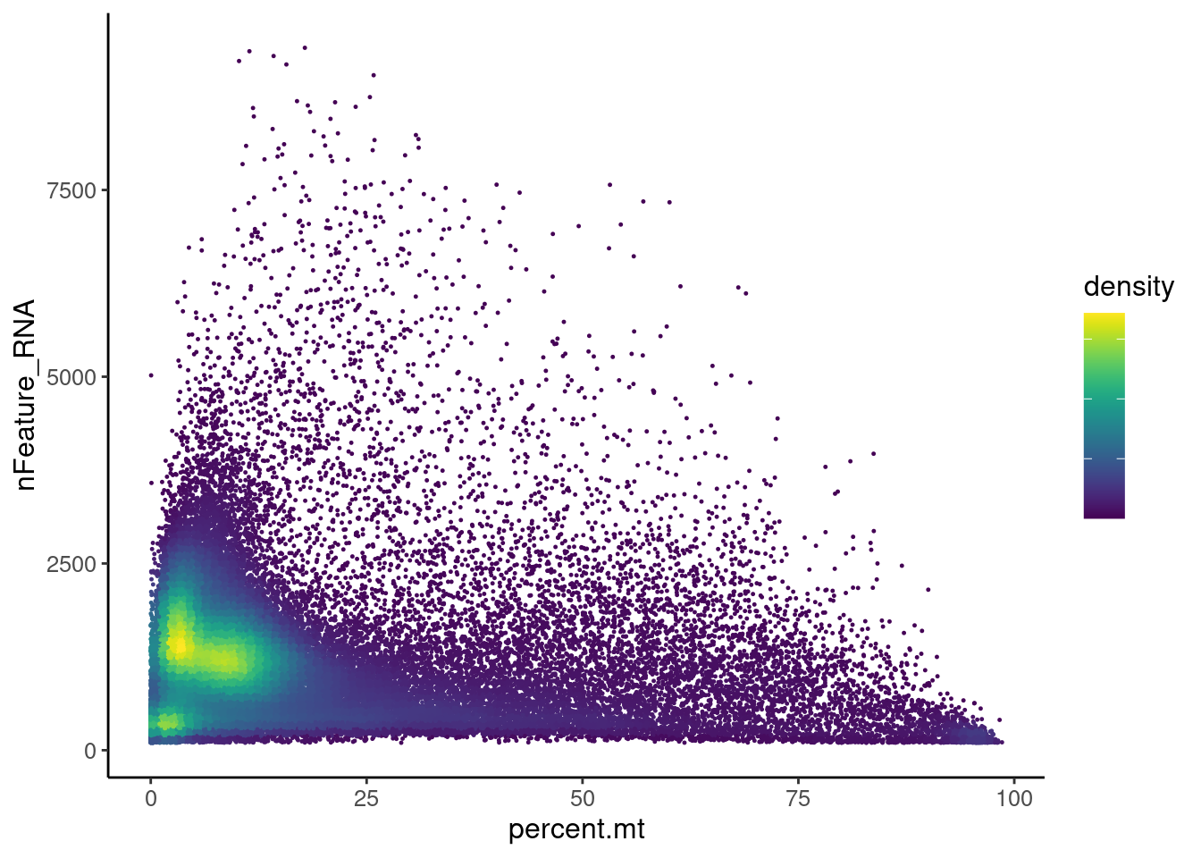
Cells >25% MT
Most cells are located between 0 and 25% MT. Nevertheless, let’s check the higher % of MT in more detail.
meta2 <- seudata@meta.data[seudata@meta.data$percent.mt > 25,]
meta2$density <- get_density(meta2$percent.mt, meta2$nFeature_RNA, n = 100)

ggplot(meta2) +
  geom_vline(xintercept = 65, color = '#7A7A7A', linetype="dashed") +
  geom_vline(xintercept = 95, color = '#7A7A7A', linetype="dashed") +
  geom_point(aes(percent.mt, nFeature_RNA, color = density), size = 0.2) +
  scale_color_viridis() + theme_classic() +
  theme(plot.title = element_text(size = 25))+
  theme(text = element_text( size = 12),
        axis.text.x = element_text( size = 10),
        axis.text.y = element_text( size = 10),
        legend.text = element_blank())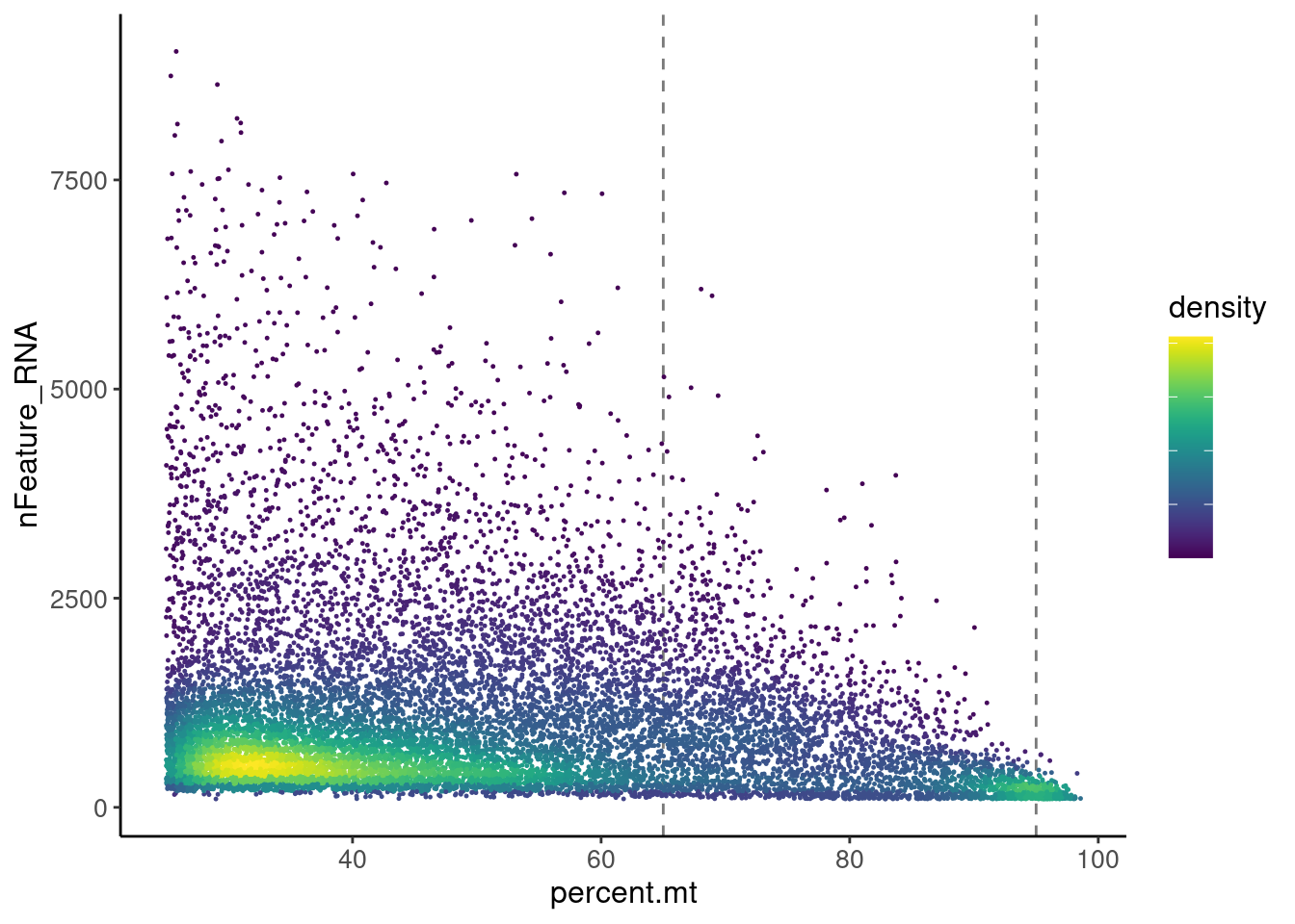
There are two main densities in the plot, one between 25 and 65, and
the second around 95%.
We keep all cells <65%MT and get rid of the density around 95%, which
will bring no information to the data set.
MT filtering
seudataf <- seudataf[,seudataf$percent.mt < 65]
seudataf
## An object of class Seurat
## 28287 features across 51056 samples within 1 assay
## Active assay: RNA (28287 features, 0 variable features)ta3 <- as.data.frame(table(seudataf$sample_name, seudataf$Health))
colnames(ta3) <- c('sample','Health','n_cells')
ta3 <- ta3[ta3$n_cells != 0,]
ta3$sample <- factor(ta3$sample, levels = c("HC 1", "HC 2", "HC 3", "HC 4",
"HC 5", "HC 6", "CD 1", "CD 2",
"CD 3", "CD 4", "CD 5", "CD 6",
"UC 1", "UC 2", "UC 3", "UC 4",
"UC 5", "UC 6"))
ggplot(data=ta3, aes(x=sample, y=n_cells, fill=Health)) +
geom_bar(stat="identity", position=position_dodge())+
geom_text(aes(label=n_cells), vjust=1.6, color="black",
position = position_dodge(0.9), size=2.5)+
scale_fill_manual(values = colors_health_alpha)+
labs(y = 'number of cells after MT filter') +
theme_classic()+
theme(axis.text.x = element_text(angle=90, vjust=0.5),
legend.title = element_blank(),
axis.title.x= element_blank())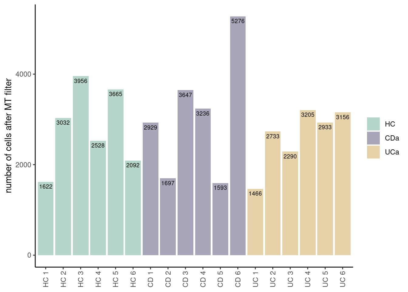
Genes without expression filtering
counts <- seudataf@assays$RNA@counts
pp <- which(Matrix::rowSums(counts)==0)
length(pp)
## [1] 278xx <-setdiff(rownames(seudataf), names(pp))
seudataf <- subset(seudataf, features = xx)
seudataf## An object of class Seurat
## 28009 features across 51056 samples within 1 assay
## Active assay: RNA (28009 features, 0 variable features)Save data as RDS file
setwd('~/000_GitHub/ibd-bcn_single_cell/')
saveRDS(seudataf, file = 'Analysis of our data/02_Samples_Together/filtered_data_together.RDS')
sessionInfo()
sessionInfo()## R version 4.1.2 (2021-11-01)
## Platform: x86_64-pc-linux-gnu (64-bit)
## Running under: Ubuntu 20.04.5 LTS
##
## Matrix products: default
## BLAS: /usr/lib/x86_64-linux-gnu/blas/libblas.so.3.9.0
## LAPACK: /opt/R/4.1.2/lib/R/lib/libRlapack.so
##
## locale:
## [1] LC_CTYPE=C.UTF-8 LC_NUMERIC=C LC_TIME=C.UTF-8 LC_COLLATE=C.UTF-8
## [5] LC_MONETARY=C.UTF-8 LC_MESSAGES=C LC_PAPER=C.UTF-8 LC_NAME=C
## [9] LC_ADDRESS=C LC_TELEPHONE=C LC_MEASUREMENT=C.UTF-8 LC_IDENTIFICATION=C
##
## attached base packages:
## [1] stats4 stats graphics grDevices utils datasets methods base
##
## other attached packages:
## [1] Matrix_1.4-0 nnet_7.3-17 matchSCore2_0.1.0 harmony_0.1.0
## [5] Rcpp_1.0.9 rmarkdown_2.18 pandoc_0.1.0 readxl_1.3.1
## [9] magick_2.7.3 data.table_1.14.2 BiocParallel_1.28.3 RColorBrewer_1.1-3
## [13] ggrepel_0.9.1 ggrastr_1.0.1 usethis_2.1.5 clustree_0.4.4
## [17] ggraph_2.0.5 readr_2.1.2 dplyr_1.0.10 cowplot_1.1.1
## [21] reshape_0.8.8 formulaic_0.0.8 patchwork_1.1.2 MASS_7.3-55
## [25] viridis_0.6.2 viridisLite_0.4.1 scDblFinder_1.8.0 scran_1.22.1
## [29] scater_1.22.0 scuttle_1.4.0 celda_1.10.0 beepr_1.3
## [33] DropletUtils_1.14.2 SingleCellExperiment_1.16.0 SummarizedExperiment_1.24.0 Biobase_2.54.0
## [37] GenomicRanges_1.46.1 GenomeInfoDb_1.30.1 IRanges_2.28.0 S4Vectors_0.32.4
## [41] BiocGenerics_0.40.0 MatrixGenerics_1.6.0 matrixStats_0.62.0 ggplot2_3.3.6
## [45] plyr_1.8.7 sp_1.5-0 SeuratObject_4.1.1 Seurat_4.1.0.9007
##
## loaded via a namespace (and not attached):
## [1] rsvd_1.0.5 ica_1.0-3 corpcor_1.6.10 assertive.properties_0.0-4
## [5] foreach_1.5.2 lmtest_0.9-40 rprojroot_2.0.3 crayon_1.5.2
## [9] spatstat.core_2.4-4 rhdf5filters_1.6.0 backports_1.4.1 nlme_3.1-155
## [13] rlang_1.0.6 XVector_0.34.0 ROCR_1.0-11 irlba_2.3.5
## [17] SparseM_1.81 limma_3.50.3 xgboost_1.5.0.2 rjson_0.2.21
## [21] bit64_4.0.5 glue_1.6.2 sctransform_0.3.4 parallel_4.1.2
## [25] vipor_0.4.5 spatstat.sparse_2.1-1 AnnotationDbi_1.56.2 spatstat.geom_2.4-0
## [29] tidyselect_1.1.2 fitdistrplus_1.1-8 tidyr_1.2.1 assertive.types_0.0-3
## [33] zoo_1.8-10 org.Mm.eg.db_3.14.0 xtable_1.8-4 magrittr_2.0.3
## [37] evaluate_0.18 cli_3.4.0 zlibbioc_1.40.0 rstudioapi_0.13
## [41] miniUI_0.1.1.1 bslib_0.4.1 rpart_4.1.16 RcppEigen_0.3.3.9.2
## [45] shiny_1.7.3 BiocSingular_1.10.0 xfun_0.34 clue_0.3-60
## [49] cluster_2.1.2 tidygraph_1.2.1 KEGGREST_1.34.0 tibble_3.1.8
## [53] listenv_0.8.0 Biostrings_2.62.0 png_0.1-7 future_1.28.0
## [57] withr_2.5.0 bitops_1.0-7 ggforce_0.3.3 cellranger_1.1.0
## [61] assertive.base_0.0-9 dqrng_0.3.0 pillar_1.8.1 GlobalOptions_0.1.2
## [65] cachem_1.0.6 fs_1.5.2 GetoptLong_1.0.5 DelayedMatrixStats_1.16.0
## [69] vctrs_0.4.1 ellipsis_0.3.2 generics_0.1.3 tools_4.1.2
## [73] beeswarm_0.4.0 munsell_0.5.0 tweenr_1.0.2 DelayedArray_0.20.0
## [77] fastmap_1.1.0 compiler_4.1.2 pkgload_1.2.4 abind_1.4-5
## [81] httpuv_1.6.6 plotly_4.10.0 rgeos_0.5-9 GenomeInfoDbData_1.2.7
## [85] gridExtra_2.3 enrichR_3.0 edgeR_3.36.0 lattice_0.20-45
## [89] deldir_1.0-6 utf8_1.2.2 later_1.3.0 jsonlite_1.8.3
## [93] multipanelfigure_2.1.2 scales_1.2.1 graph_1.72.0 ScaledMatrix_1.2.0
## [97] pbapply_1.5-0 sparseMatrixStats_1.6.0 lazyeval_0.2.2 promises_1.2.0.1
## [101] doParallel_1.0.17 R.utils_2.12.0 goftest_1.2-3 checkmate_2.0.0
## [105] spatstat.utils_2.3-1 reticulate_1.26 textshaping_0.3.6 statmod_1.4.36
## [109] Rtsne_0.16 uwot_0.1.14 igraph_1.3.4 HDF5Array_1.22.1
## [113] survival_3.2-13 rsconnect_0.8.25 yaml_2.3.6 systemfonts_1.0.4
## [117] htmltools_0.5.3 memoise_2.0.1 locfit_1.5-9.6 graphlayouts_0.8.0
## [121] digest_0.6.30 assertthat_0.2.1 rappdirs_0.3.3 mime_0.12
## [125] RSQLite_2.2.17 future.apply_1.9.1 blob_1.2.3 R.oo_1.25.0
## [129] ragg_1.2.1 splines_4.1.2 labeling_0.4.2 Rhdf5lib_1.16.0
## [133] RCurl_1.98-1.8 assertive.numbers_0.0-2 hms_1.1.1 rhdf5_2.38.1
## [137] colorspace_2.0-3 ggbeeswarm_0.6.0 shape_1.4.6 assertive.files_0.0-2
## [141] sass_0.4.2 RANN_2.6.1 circlize_0.4.14 audio_0.1-10
## [145] fansi_1.0.3 tzdb_0.2.0 brio_1.1.3 parallelly_1.32.1
## [149] R6_2.5.1 grid_4.1.2 ggridges_0.5.3 lifecycle_1.0.3
## [153] formatR_1.12 bluster_1.4.0 curl_4.3.2 jquerylib_0.1.4
## [157] leiden_0.4.3 testthat_3.1.2 desc_1.4.0 RcppAnnoy_0.0.19
## [161] org.Hs.eg.db_3.14.0 iterators_1.0.14 stringr_1.4.1 topGO_2.46.0
## [165] htmlwidgets_1.5.4 beachmat_2.10.0 polyclip_1.10-0 purrr_0.3.4
## [169] gridGraphics_0.5-1 ComplexHeatmap_2.10.0 mgcv_1.8-38 globals_0.16.1
## [173] spatstat.random_2.2-0 progressr_0.11.0 codetools_0.2-18 GO.db_3.14.0
## [177] metapod_1.2.0 MCMCprecision_0.4.0 R.methodsS3_1.8.2 gtable_0.3.1
## [181] DBI_1.1.3 highr_0.9 tensor_1.5 httr_1.4.4
## [185] KernSmooth_2.23-20 vroom_1.5.7 stringi_1.7.8 reshape2_1.4.4
## [189] farver_2.1.1 combinat_0.0-8 BiocNeighbors_1.12.0 scattermore_0.8
## [193] bit_4.0.4 spatstat.data_2.2-0 pkgconfig_2.0.3 corrplot_0.92
## [197] knitr_1.40