Epithelium subset analysis
Last compiled on 17 November, 2022
We considered five major cell subsets: (1) myeloid, (2) T, (3) B and plasma, (4) stromal, and (5) epithelial cells. We classified cells into these subsets according to their gene expression. We consider in this file the cells classified as epithelium. We reanalyze and QC the data,and look for the refined clusters.
Load libraries
library(Seurat)
library(plyr)
library(dplyr)
library(ggplot2)
library(DropletUtils)
library(celda)
library(SingleCellExperiment)
library(scater)
library(scran)
library(scDblFinder)
library(viridis)
library(MASS)
library(patchwork)
library(readr)
library(clustree)
Load extra functions and sources
get_density <- function(x, y, ...) { # function from https://slowkow.com/notes/ggplot2-color-by-density/
  dens <- MASS::kde2d(x, y, ...)
  ix <- findInterval(x, dens$x)
  iy <- findInterval(y, dens$y)
  ii <- cbind(ix, iy)
  return(dens$z[ii])
}

fancy_scientific <- function(l) { # function from https://stackoverflow.com/a/24241954
     # turn in to character string in scientific notation
     l <- format(l, scientific = TRUE)
     # quote the part before the exponent to keep all the digits
     l <- gsub("^(.*)e", "'\\1'e", l)
     # turn the 'e+' into plotmath format
     l <- gsub("e", "%*%10^", l)
     # return this as an expression
     parse(text=l)
}

setwd("~/000_GitHub/ibd-bcn_single_cell")
source('source/functions_scrnaseq.R')
source('source/colors.R')
Load the data
setwd('~/000_GitHub/ibd-bcn_single_cell/Analysis of our data/02_Samples_Together/')
epi <- readRDS('SUBSETS/FROM_SAMPLES_TOGETHER/epi.RDS')
Reanalysis
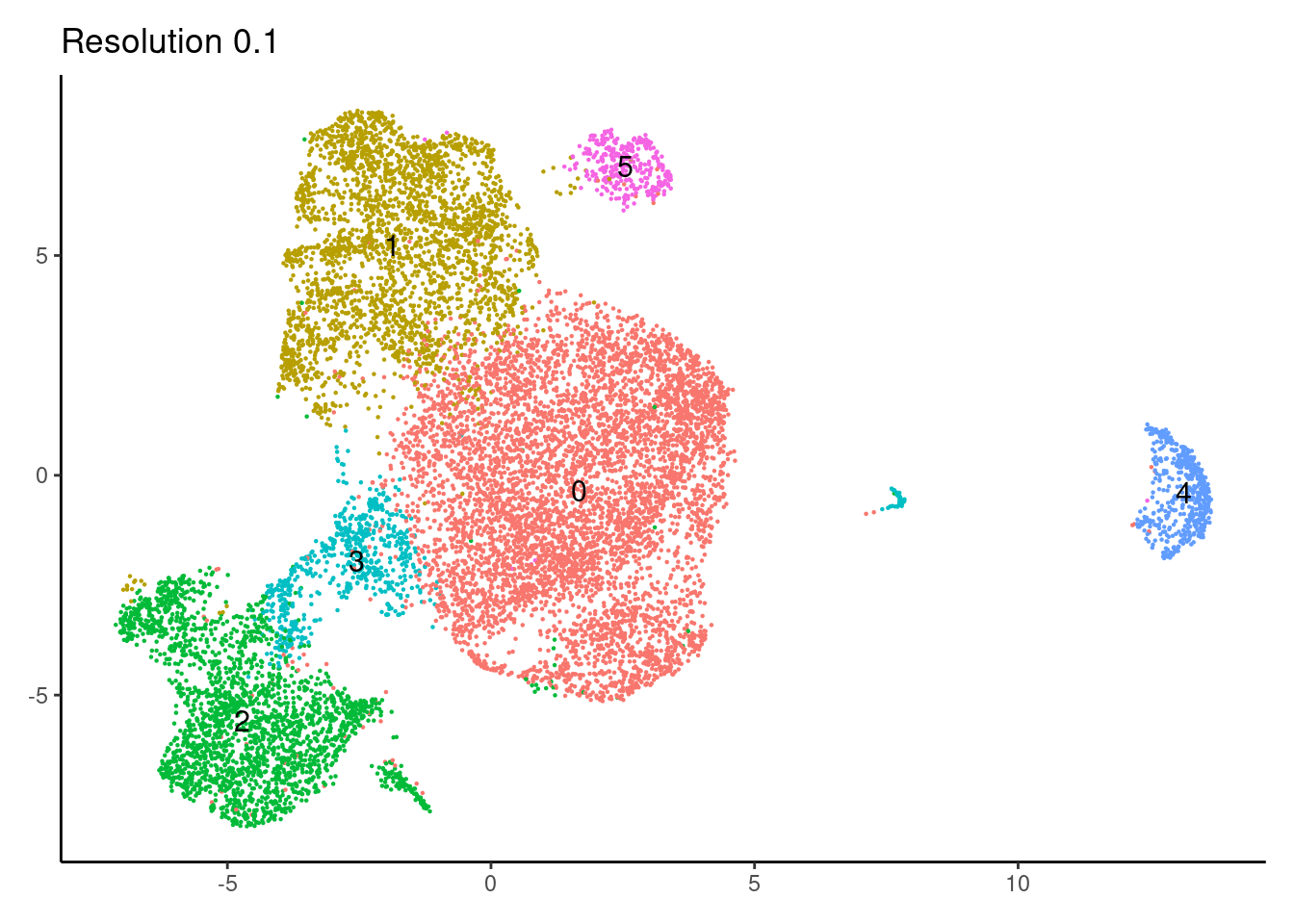
These are the clusters we selected as epithelial in the “02_Data_to_subsets” file.
DimPlot(epi, label=T, group.by = 'RNA_snn_res.0.1')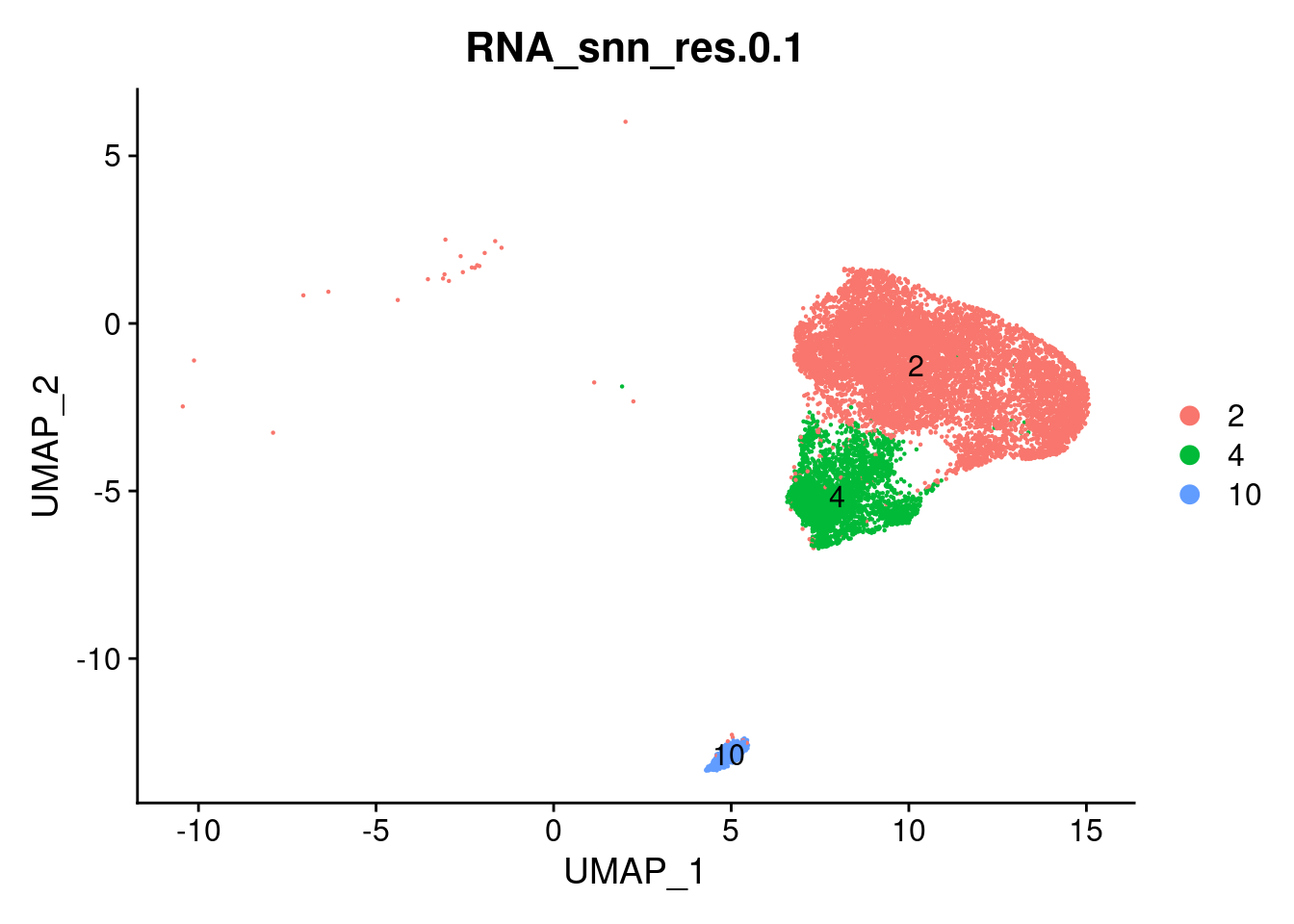
QC
MT-gene expression
Distribution of cells in scatter plot (nfeatures/percent.mt) to check where are the majority of our cells. We can see the dots colored by density using the function get_density shown in Load extra functions and sources.
meta <- epi@meta.data
meta$density <- get_density(meta$percent.mt, meta$nFeature_RNA, n = 100)
ggplot(meta) +
  geom_point(aes(percent.mt, nFeature_RNA, color = density), size = 0.2) +
  scale_color_viridis() + theme_classic() +
  scale_y_log10()+
  geom_vline(xintercept = 65, linetype = 2, color = 'gray')+
  theme(text = element_text( size = 12),
        axis.title = element_text( size = 12),
        legend.text = element_blank())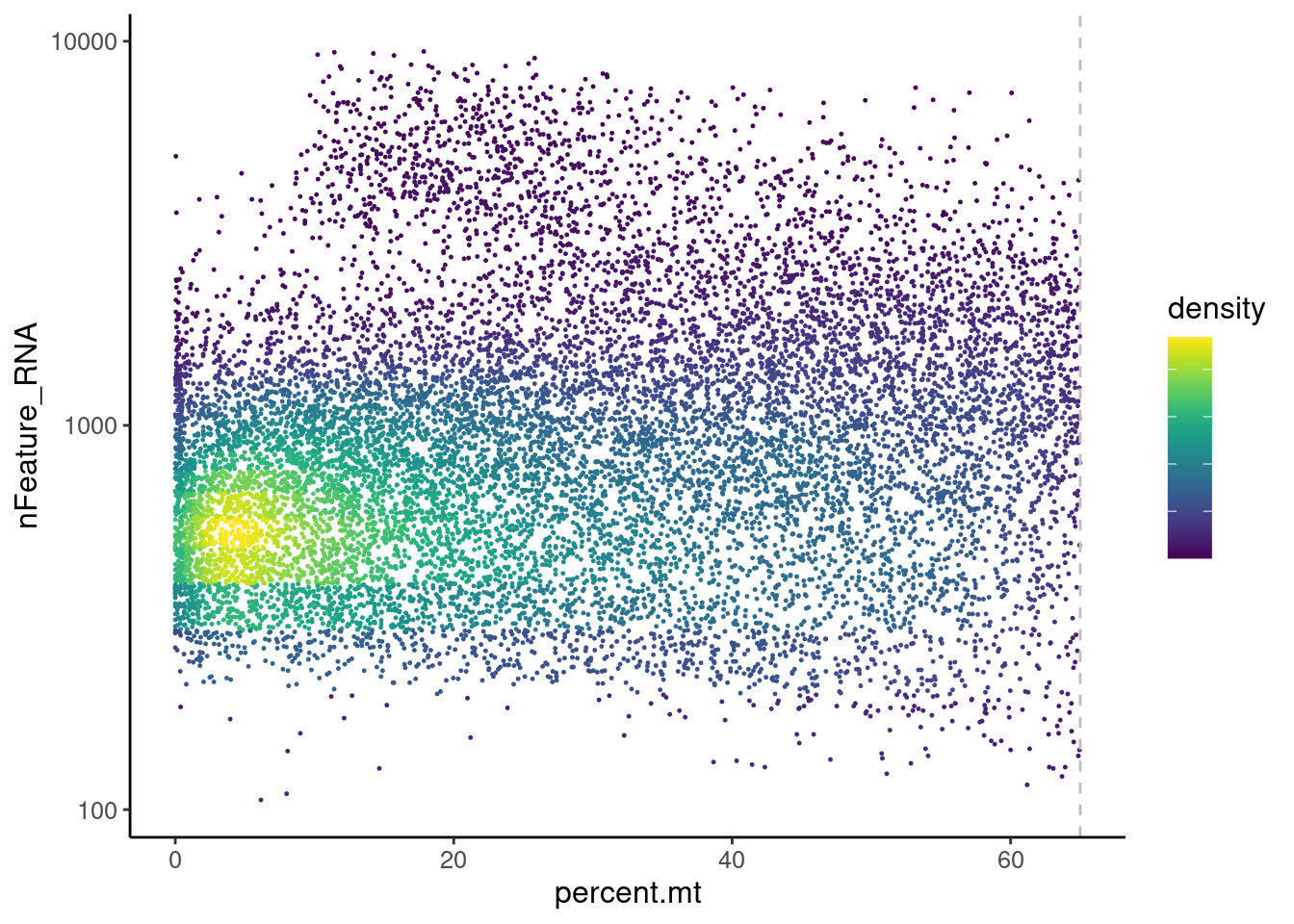
We analyzed the data using different cutoffs for the percent.mt (data not shown) and finally decided that 65% was a reasonable choice for this dataset.
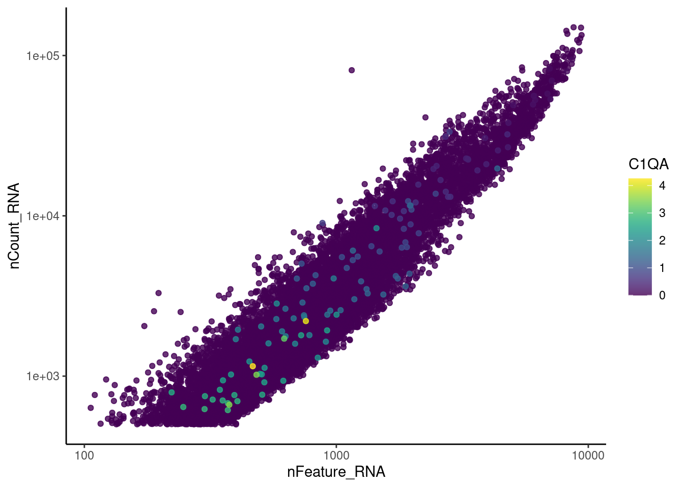
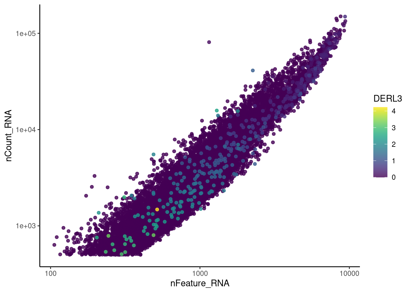
Non-epithelial genes
Right now epi has 28287 features across 12999 cells.
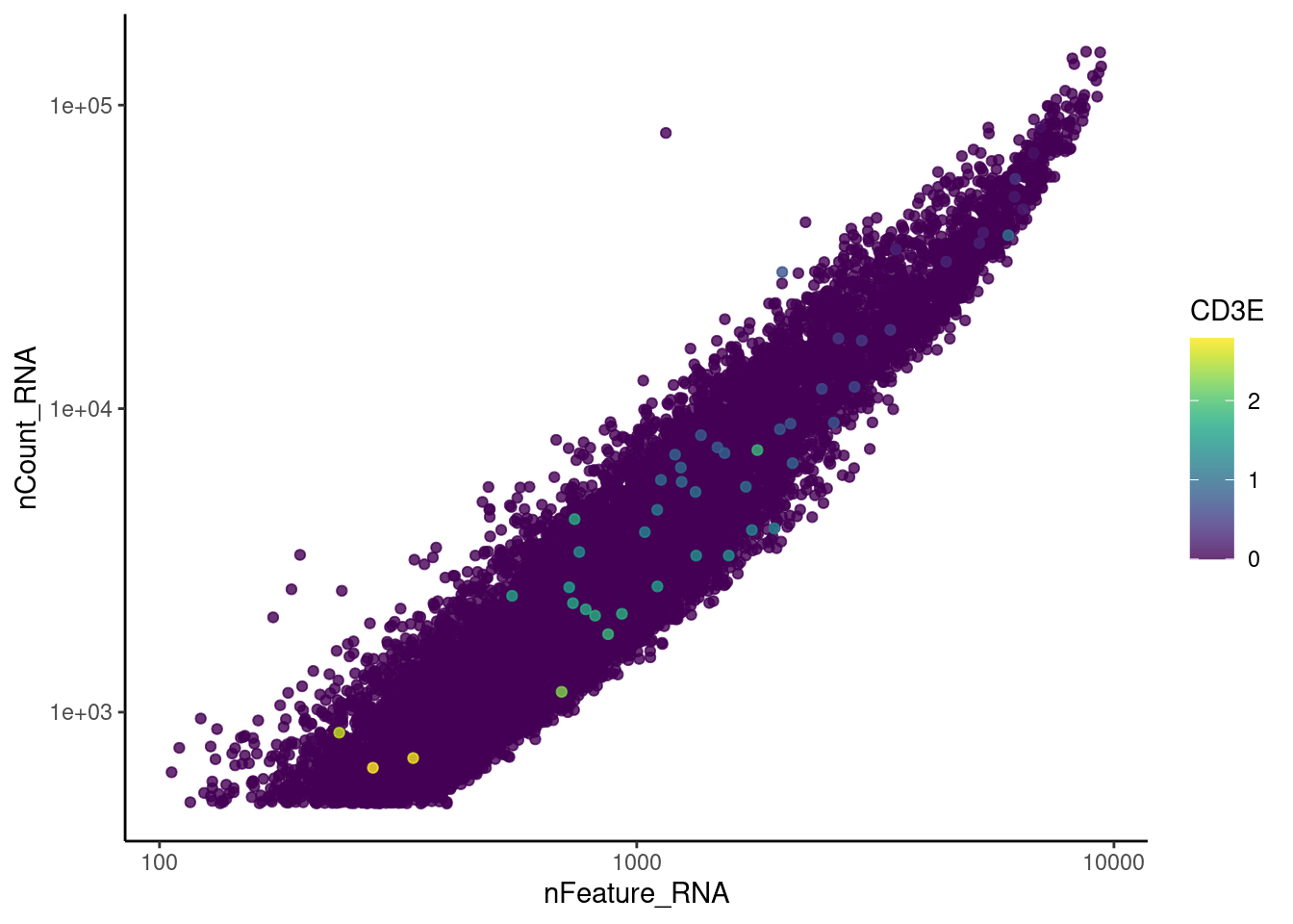
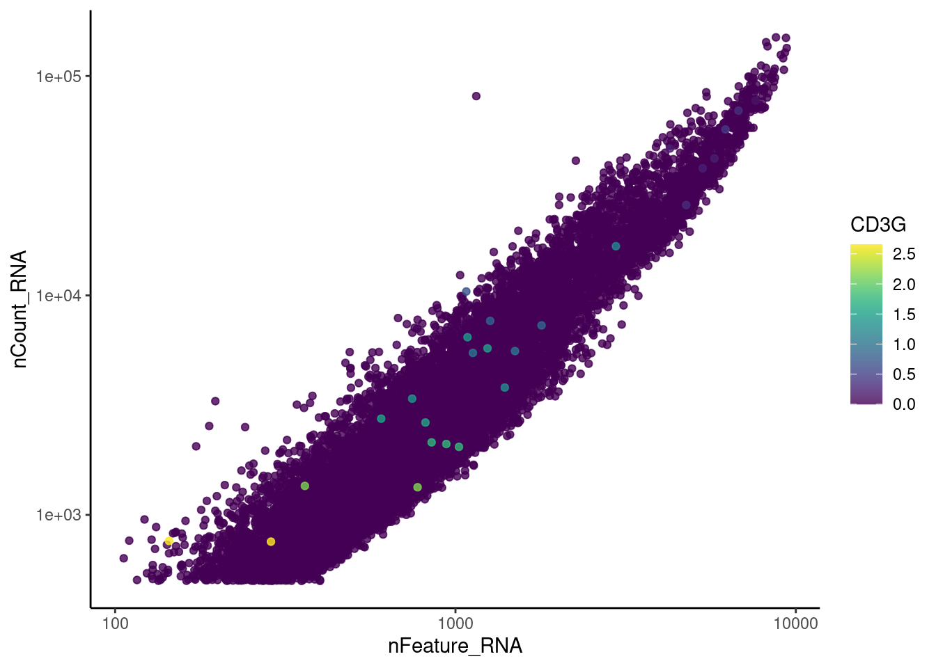
Nevertheless, many cells express genes that we know should not be
expressed by epithelial cells. We will remove those cells.
genes <-  c('CD3E','CD3D','CD3G', 'C1QA', 'DERL3', 'MS4A1')
for (gene in genes) {
    jd <- FetchData(epi, vars = c('nCount_RNA', 'nFeature_RNA', gene))
    jd <- jd[order(jd[,ncol(jd)]),]
    k <- ggplot(jd, mapping = aes_string(x = 'nFeature_RNA', y = 'nCount_RNA', color = gene))+
      geom_point() + theme_classic() + scale_color_viridis(alpha = 0.8) + scale_y_log10() + scale_x_log10()
    cat("#### ", gene, "\n"); print(k); cat("\n\n")
  }
CD3E
CD3D

CD3G
C1QA
DERL3
MS4A1

cat("#### code removal \n")code removal
counts <- epi@assays$RNA@counts
p <- grep("CD3E$|CD3D$|CD3G$|MS4A1$|DERL3|^C1QA$",rownames(epi))
pp <- which(Matrix::colSums(counts[p,])>0)
xx <-setdiff(colnames(epi), names(pp))
epi <- subset(epi,cells = xx)
cat('\n\n')
Ig genes signal
We have observed that due to normalization, there’s high Ig gene expression in cells that did not have high counts of Ig genes. As an example:
a <- FeaturePlot(epi, features = 'IGHA1', slot = 'counts') + labs(title='counts') + theme_classic()
b <- FeaturePlot(epi, features = 'IGHA1', slot = 'data') + labs(title= 'data') + theme_classic()
wrap_plots(a,b, nrow = 1)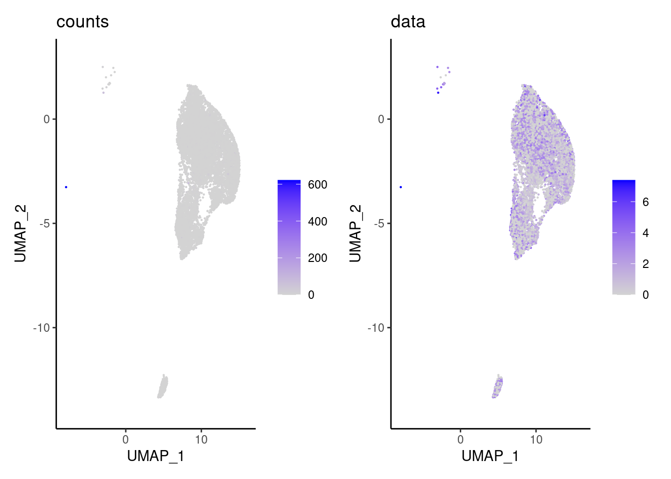
We remove the Ig genes from the dataset in all subsets except for the plasma and B cells subset.
gg <- rownames(epi)[c(grep("^IGH",rownames(epi)),
                         grep("^IGK", rownames(epi)),
                         grep("^IGL", rownames(epi)))]
genes <- setdiff(rownames(epi),gg)
epi <- subset(epi,features = genes)
Genes without expression
We remove the genes without expression from the dataset.
counts <- epi@assays$RNA@counts
pp <- which(Matrix::rowSums(counts)==0)
xx <-setdiff(rownames(epi), names(pp))
epi <- subset(epi, features = xx)
Dimension reduction
epi <- seurat_to_pca(epi)

a <- ElbowPlot(epi, ndims = 100) +
  geom_vline(xintercept = 22, colour="#BB0000", linetype = 2)+
  labs(title = paste0('Elbowplot')) + theme_classic()

epi<- FindNeighbors(epi, dims = 1:22)
epi<-RunUMAP(epi, dims=1:22)
b <- DimPlot(epi, group.by = 'sample_name') +
  labs(title = '22 PCS') +
  theme_classic() +
  theme(legend.position = 'bottom')

(a+b) / guide_area() +
  plot_layout(heights = c(0.7,0.3),guides = 'collect')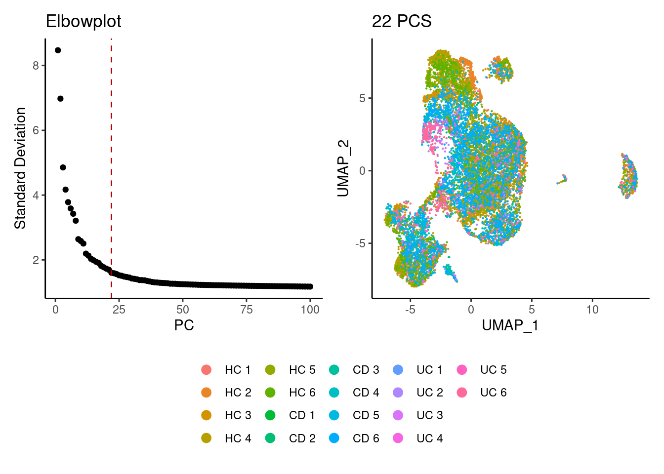
Louvain Clusterization
# dir.create('Markers')
# dir.create('Markers/Epithelium')
path <- '~/000_GitHub/ibd-bcn_single_cell/Analysis of our data/02_Samples_Together/SUBSETS/Markers'
setwd(path)
epi <- resolutions(epi,
                   workingdir = path,
                   title = 'Epithelium/Markers_Epithelium_')
path <- '~/000_GitHub/ibd-bcn_single_cell/Analysis of our data/02_Samples_Together/SUBSETS/ON_THEIR_OWN/'
setwd(path)
saveRDS(epi, file = paste0(path,'epi_filtered.RDS'))
Dimplot Resolutions
path <- '~/000_GitHub/ibd-bcn_single_cell/Analysis of our data/02_Samples_Together/SUBSETS/ON_THEIR_OWN/'
epi <- readRDS(file = paste0(path,'epi_filtered.RDS'))
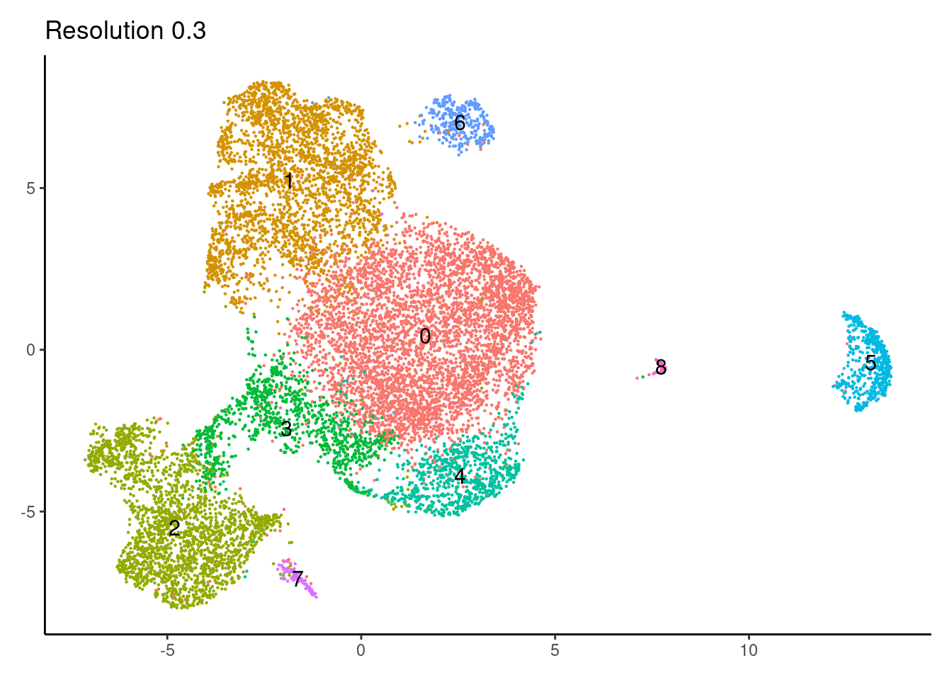
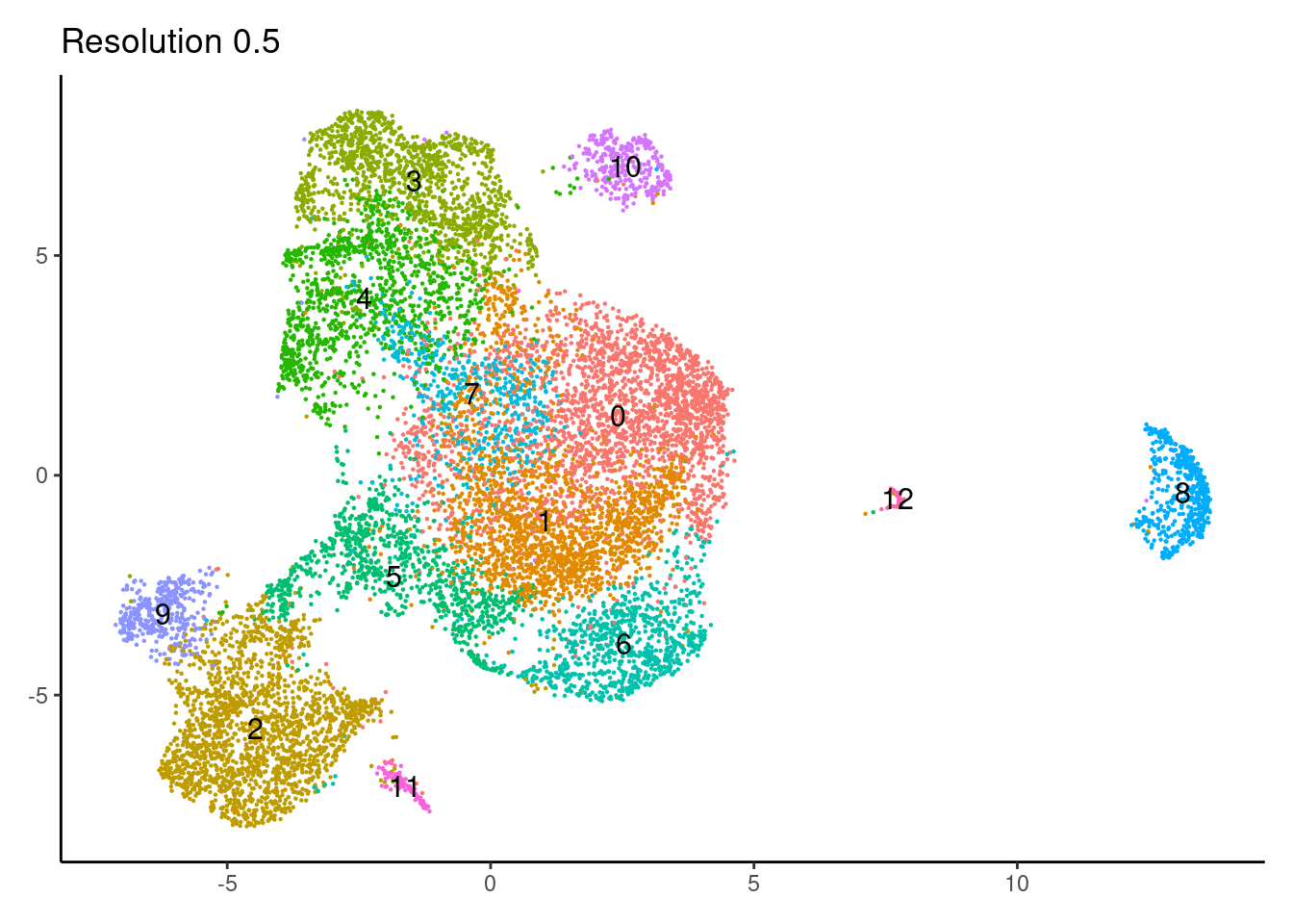
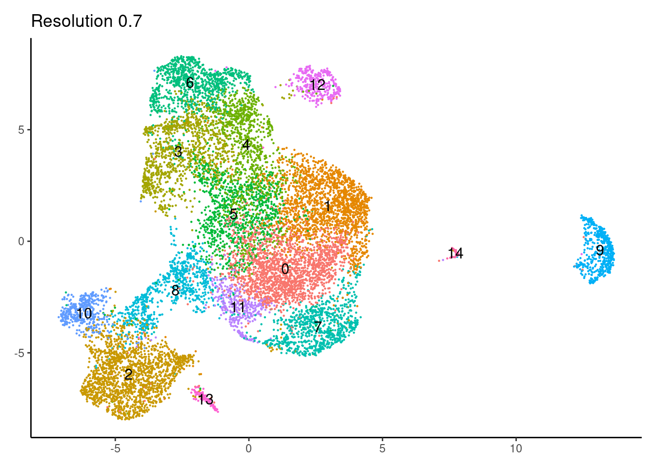
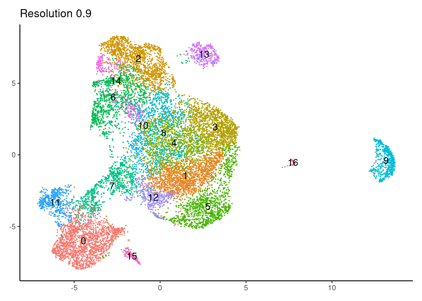
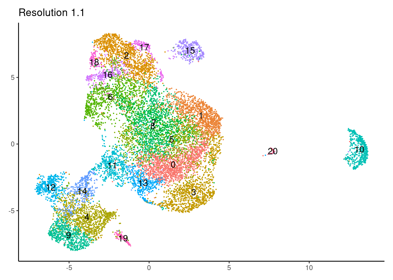
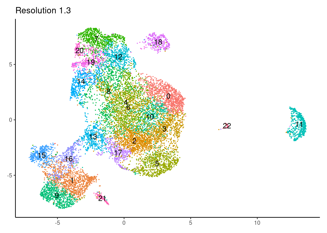
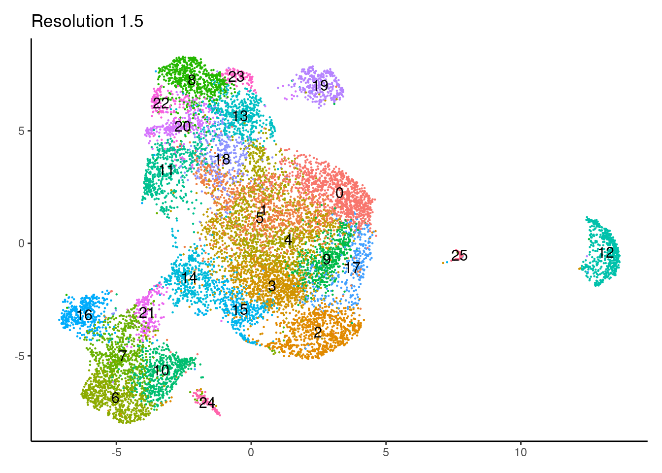
for(i in c('0.1','0.3','0.5','0.7','0.9','1.1','1.3','1.5')){
j <-DimPlot(epi, group.by = paste0('RNA_snn_res.',i), label=T) +
theme_classic() +
theme(legend.position = 'none', axis.title = element_blank()) +
labs(title = paste0('Resolution ',i))
cat("##### ", i, "\n"); print(j); cat("\n\n")
}0.1
0.3
0.5
0.7
0.9
1.1
1.3
1.5
Clustree Resolutions
clustree(epi, prefix = 'RNA_snn_res.') + guides(size = 'none', shape = 'none', edge_colour = FALSE, edge_alpha = FALSE) + theme(legend.position = 'right')## Warning: `guides(<scale> = FALSE)` is deprecated. Please use `guides(<scale> = "none")` instead.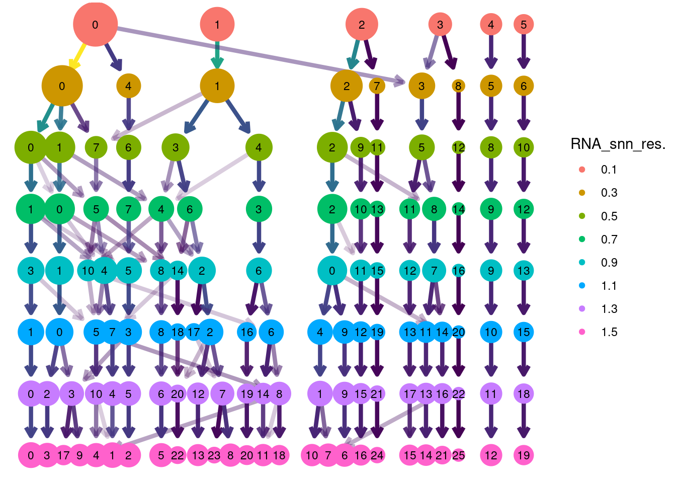
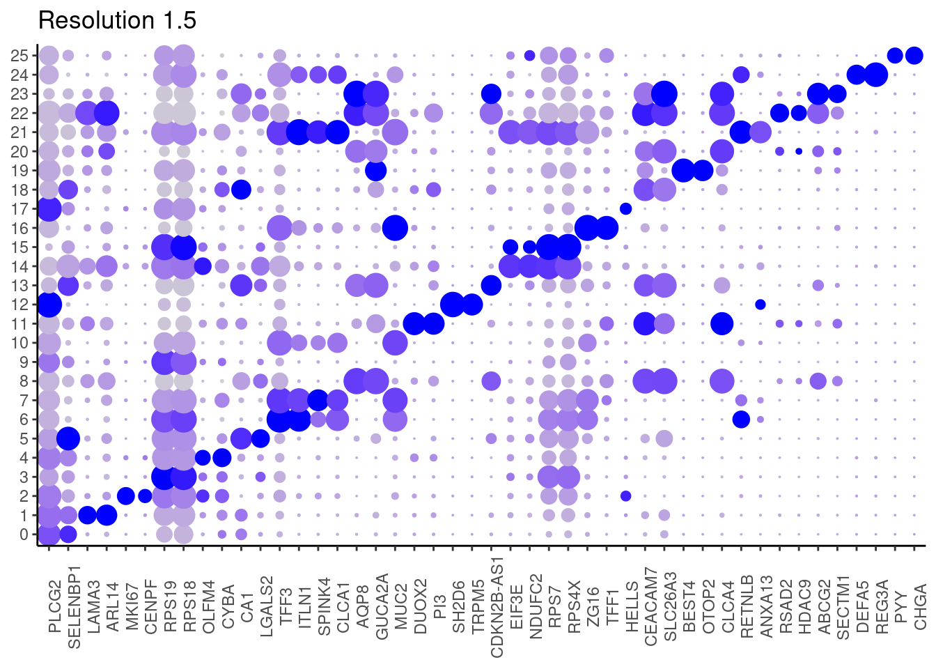
Top2 markers
setwd('~/000_GitHub/ibd-bcn_single_cell/Analysis of our data/02_Samples_Together/SUBSETS/')
for(i in c('0.1','0.3','0.5','0.7','0.9','1.1','1.3','1.5')){
  marker_genes <- read_delim(
    paste0("Markers/Epithelium/Markers_Epithelium__markers_resolution_",i,".csv"),
    delim = ";", escape_double = FALSE, locale = locale(decimal_mark = ",",
                                                        grouping_mark = "."), trim_ws = TRUE)

  top2 <- marker_genes %>%
    dplyr::group_by(cluster)%>%
    dplyr::slice(1:2)
  top2_g <- unique(top2$gene)

  j <- DotPlot(epi, features = top2_g, group.by = paste0('RNA_snn_res.', i)) +
    theme_classic() +
    theme(axis.text.x = element_text(angle=90),
          axis.title = element_blank()) +
    NoLegend() +
    labs(title = paste0('Resolution ',i))
  cat("##### ", i, "\n"); print(j); cat("\n\n")
}
## Rows: 2738 Columns: 7
## ── Column specification ──────────────────────────────────────────────────────────────────────────────────────────────
## Delimiter: ";"
## chr (1): gene
## dbl (6): p_val, avg_log2FC, pct.1, pct.2, p_val_adj, cluster
##
## ℹ Use `spec()` to retrieve the full column specification for this data.
## ℹ Specify the column types or set `show_col_types = FALSE` to quiet this message.0.1
## Rows: 3404 Columns: 7
## ── Column specification ──────────────────────────────────────────────────────────────────────────────────────────────
## Delimiter: ";"
## chr (1): gene
## dbl (6): p_val, avg_log2FC, pct.1, pct.2, p_val_adj, cluster
##
## ℹ Use `spec()` to retrieve the full column specification for this data.
## ℹ Specify the column types or set `show_col_types = FALSE` to quiet this message.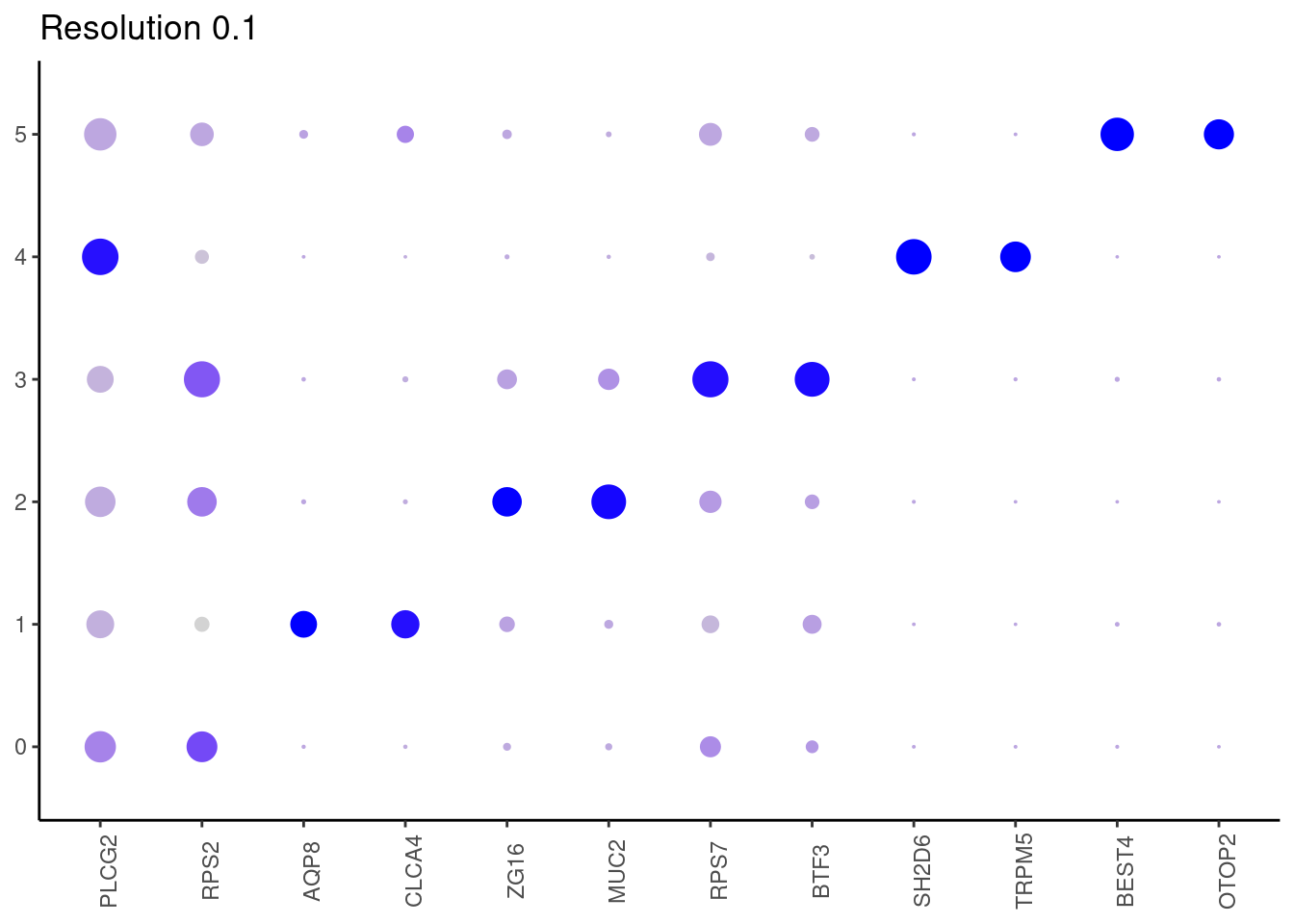 #####
0.3
#####
0.3
## Rows: 5222 Columns: 7
## ── Column specification ──────────────────────────────────────────────────────────────────────────────────────────────
## Delimiter: ";"
## chr (1): gene
## dbl (6): p_val, avg_log2FC, pct.1, pct.2, p_val_adj, cluster
##
## ℹ Use `spec()` to retrieve the full column specification for this data.
## ℹ Specify the column types or set `show_col_types = FALSE` to quiet this message.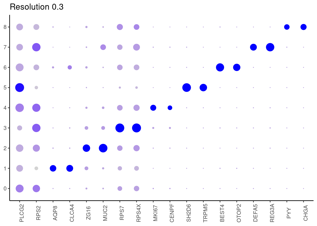 #####
0.5
#####
0.5
## Rows: 6116 Columns: 7
## ── Column specification ──────────────────────────────────────────────────────────────────────────────────────────────
## Delimiter: ";"
## chr (1): gene
## dbl (6): p_val, avg_log2FC, pct.1, pct.2, p_val_adj, cluster
##
## ℹ Use `spec()` to retrieve the full column specification for this data.
## ℹ Specify the column types or set `show_col_types = FALSE` to quiet this message.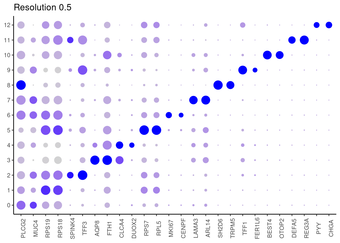 #####
0.7
#####
0.7
## Rows: 6976 Columns: 7
## ── Column specification ──────────────────────────────────────────────────────────────────────────────────────────────
## Delimiter: ";"
## chr (1): gene
## dbl (6): p_val, avg_log2FC, pct.1, pct.2, p_val_adj, cluster
##
## ℹ Use `spec()` to retrieve the full column specification for this data.
## ℹ Specify the column types or set `show_col_types = FALSE` to quiet this message.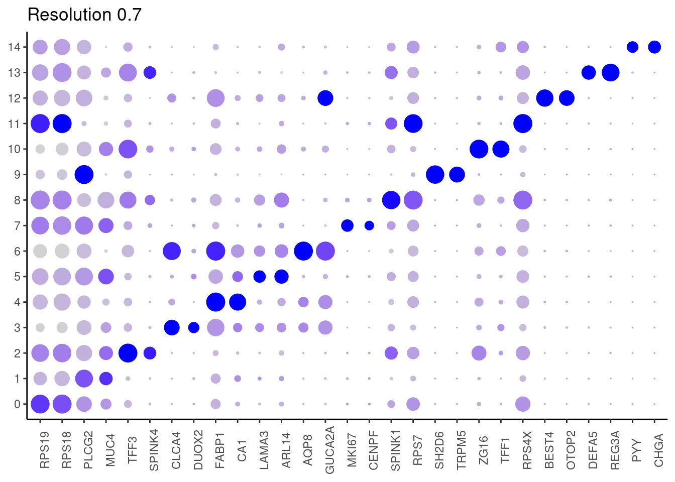 #####
0.9
#####
0.9
## Rows: 9302 Columns: 7
## ── Column specification ──────────────────────────────────────────────────────────────────────────────────────────────
## Delimiter: ";"
## chr (1): gene
## dbl (6): p_val, avg_log2FC, pct.1, pct.2, p_val_adj, cluster
##
## ℹ Use `spec()` to retrieve the full column specification for this data.
## ℹ Specify the column types or set `show_col_types = FALSE` to quiet this message.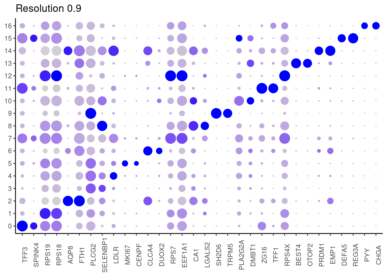 #####
1.1
#####
1.1
## Rows: 9857 Columns: 7
## ── Column specification ──────────────────────────────────────────────────────────────────────────────────────────────
## Delimiter: ";"
## chr (1): gene
## dbl (6): p_val, avg_log2FC, pct.1, pct.2, p_val_adj, cluster
##
## ℹ Use `spec()` to retrieve the full column specification for this data.
## ℹ Specify the column types or set `show_col_types = FALSE` to quiet this message.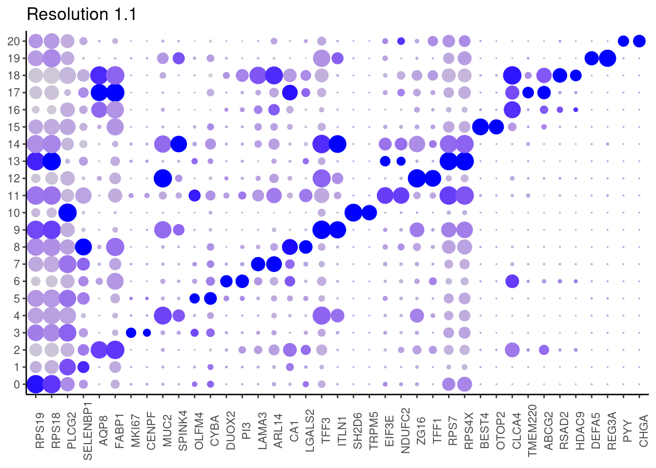 #####
1.3
#####
1.3
## Rows: 11316 Columns: 7
## ── Column specification ──────────────────────────────────────────────────────────────────────────────────────────────
## Delimiter: ";"
## chr (1): gene
## dbl (6): p_val, avg_log2FC, pct.1, pct.2, p_val_adj, cluster
##
## ℹ Use `spec()` to retrieve the full column specification for this data.
## ℹ Specify the column types or set `show_col_types = FALSE` to quiet this message.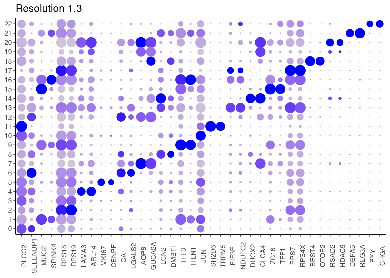 #####
1.5
#####
1.5
Annotation
epi$annotation_refined <- plyr::mapvalues(x = epi$RNA_snn_res.0.7,
                                               from = 0:14,
                                               to = c("Epithelium Ribhi",
                                                      "PLCG2 colonocytes",
                                                      "Goblet",
                                                      "Inflammatory colonocyte",
                                                      "Colonocyte 1",
                                                      "Laminin colonocytes",
                                                      "Colonocyte 2",
                                                      "Cycling TA",
                                                      "Secretory progenitor",
                                                      "Tuft cells",
                                                      "Mature goblet",
                                                      "Epithelium Ribhi",
                                                      "BEST4 OTOP2",
                                                      "Paneth-like",
                                                      "Enteroendocrine")


)

epi$annotation_intermediate <- plyr::mapvalues(x = epi$RNA_snn_res.0.7,
                                               from = 0:14,
                                               to = c("Epithelium Ribhi",
                                                      "Colonocytes",
                                                      "Goblet",
                                                      "Inflammatory colonocyte",
                                                      "Colonocytes",
                                                      "Colonocytes",
                                                      "Colonocytes",
                                                      "Cycling TA",
                                                      "Secretory progenitor",
                                                      "Tuft cells",
                                                      "Goblet",
                                                      "Epithelium Ribhi",
                                                      "BEST4 OTOP2",
                                                      "Paneth-like",
                                                      "Enteroendocrine")

)

a <- DimPlot(epi, group.by = 'annotation_intermediate', label = T, repel=T) + NoLegend()
b <- DimPlot(epi, group.by = 'annotation_refined', label = T, repel=T, cols = cols_epi) +
  NoLegend()
a+b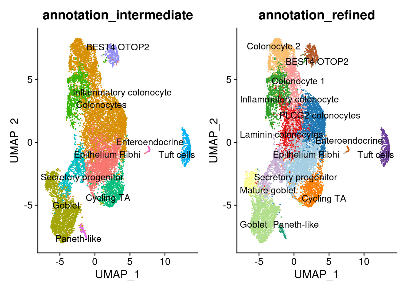
Save file
saveRDS(epi, file = '~/000_GitHub/ibd-bcn_single_cell/Analysis of our data/02_Samples_Together/SUBSETS/ON_THEIR_OWN/epi_annotated.RDS')

head(epi@meta.data)
## orig.ident nCount_RNA nFeature_RNA sample doublet Health sample_name Health_2 percent.mt
## SC_002_AAAGATGTCGAATCCA-1 SC 556 226 SC_002 singlet HC HC 1 HC 30.84577
## SC_002_AAAGTAGAGAGGTACC-1 SC 862 420 SC_002 singlet HC HC 1 HC 24.85616
## SC_002_AAAGTAGAGCCGATTT-1 SC 2478 553 SC_002 singlet HC HC 1 HC 11.77413
## SC_002_AACCGCGTCGGAATCT-1 SC 1536 675 SC_002 singlet HC HC 1 HC 11.73800
## SC_002_AACTCAGCACCCTATC-1 SC 2488 633 SC_002 singlet HC HC 1 HC 56.04000
## SC_002_AACTGGTCAGTATCTG-1 SC 2665 757 SC_002 singlet HC HC 1 HC 40.01493
## RNA_snn_res.0.1 seurat_clusters RNA_snn_res.0.3 RNA_snn_res.0.5 RNA_snn_res.0.7
## SC_002_AAAGATGTCGAATCCA-1 2 6 2 2 2
## SC_002_AAAGTAGAGAGGTACC-1 4 12 5 8 9
## SC_002_AAAGTAGAGCCGATTT-1 2 16 2 9 10
## SC_002_AACCGCGTCGGAATCT-1 0 5 0 1 0
## SC_002_AACTCAGCACCCTATC-1 4 12 5 8 9
## SC_002_AACTGGTCAGTATCTG-1 2 10 2 2 2
## RNA_snn_res.0.9 RNA_snn_res.1.1 RNA_snn_res.1.3 RNA_snn_res.1.5 annotation_refined
## SC_002_AAAGATGTCGAATCCA-1 0 9 9 6 Goblet
## SC_002_AAAGTAGAGAGGTACC-1 9 10 11 12 Tuft cells
## SC_002_AAAGTAGAGCCGATTT-1 11 12 15 16 Mature goblet
## SC_002_AACCGCGTCGGAATCT-1 1 8 6 5 Epithelium Ribhi
## SC_002_AACTCAGCACCCTATC-1 9 10 11 12 Tuft cells
## SC_002_AACTGGTCAGTATCTG-1 0 4 1 10 Goblet
## annotation_intermediate
## SC_002_AAAGATGTCGAATCCA-1 Goblet
## SC_002_AAAGTAGAGAGGTACC-1 Tuft cells
## SC_002_AAAGTAGAGCCGATTT-1 Goblet
## SC_002_AACCGCGTCGGAATCT-1 Epithelium Ribhi
## SC_002_AACTCAGCACCCTATC-1 Tuft cells
## SC_002_AACTGGTCAGTATCTG-1 GobletsessionInfo()
sessionInfo()## R version 4.1.2 (2021-11-01)
## Platform: x86_64-pc-linux-gnu (64-bit)
## Running under: Ubuntu 20.04.5 LTS
##
## Matrix products: default
## BLAS: /usr/lib/x86_64-linux-gnu/blas/libblas.so.3.9.0
## LAPACK: /opt/R/4.1.2/lib/R/lib/libRlapack.so
##
## locale:
## [1] LC_CTYPE=C.UTF-8 LC_NUMERIC=C LC_TIME=C.UTF-8 LC_COLLATE=C.UTF-8
## [5] LC_MONETARY=C.UTF-8 LC_MESSAGES=C LC_PAPER=C.UTF-8 LC_NAME=C
## [9] LC_ADDRESS=C LC_TELEPHONE=C LC_MEASUREMENT=C.UTF-8 LC_IDENTIFICATION=C
##
## attached base packages:
## [1] stats4 stats graphics grDevices utils datasets methods base
##
## other attached packages:
## [1] Matrix_1.4-0 nnet_7.3-17 matchSCore2_0.1.0 harmony_0.1.0
## [5] Rcpp_1.0.9 rmarkdown_2.18 pandoc_0.1.0 readxl_1.3.1
## [9] magick_2.7.3 data.table_1.14.2 BiocParallel_1.28.3 RColorBrewer_1.1-3
## [13] ggrepel_0.9.1 ggrastr_1.0.1 usethis_2.1.5 clustree_0.4.4
## [17] ggraph_2.0.5 readr_2.1.2 dplyr_1.0.10 cowplot_1.1.1
## [21] reshape_0.8.8 formulaic_0.0.8 patchwork_1.1.2 MASS_7.3-55
## [25] viridis_0.6.2 viridisLite_0.4.1 scDblFinder_1.8.0 scran_1.22.1
## [29] scater_1.22.0 scuttle_1.4.0 celda_1.10.0 beepr_1.3
## [33] DropletUtils_1.14.2 SingleCellExperiment_1.16.0 SummarizedExperiment_1.24.0 Biobase_2.54.0
## [37] GenomicRanges_1.46.1 GenomeInfoDb_1.30.1 IRanges_2.28.0 S4Vectors_0.32.4
## [41] BiocGenerics_0.40.0 MatrixGenerics_1.6.0 matrixStats_0.62.0 ggplot2_3.3.6
## [45] plyr_1.8.7 sp_1.5-0 SeuratObject_4.1.1 Seurat_4.1.0.9007
##
## loaded via a namespace (and not attached):
## [1] rsvd_1.0.5 ica_1.0-3 corpcor_1.6.10 assertive.properties_0.0-4
## [5] foreach_1.5.2 lmtest_0.9-40 rprojroot_2.0.3 crayon_1.5.2
## [9] spatstat.core_2.4-4 rhdf5filters_1.6.0 backports_1.4.1 nlme_3.1-155
## [13] rlang_1.0.6 XVector_0.34.0 ROCR_1.0-11 irlba_2.3.5
## [17] SparseM_1.81 limma_3.50.3 xgboost_1.5.0.2 rjson_0.2.21
## [21] bit64_4.0.5 glue_1.6.2 sctransform_0.3.4 parallel_4.1.2
## [25] vipor_0.4.5 spatstat.sparse_2.1-1 AnnotationDbi_1.56.2 spatstat.geom_2.4-0
## [29] tidyselect_1.1.2 fitdistrplus_1.1-8 tidyr_1.2.1 assertive.types_0.0-3
## [33] zoo_1.8-10 org.Mm.eg.db_3.14.0 xtable_1.8-4 magrittr_2.0.3
## [37] evaluate_0.18 cli_3.4.0 zlibbioc_1.40.0 rstudioapi_0.13
## [41] miniUI_0.1.1.1 bslib_0.4.1 rpart_4.1.16 RcppEigen_0.3.3.9.2
## [45] shiny_1.7.3 BiocSingular_1.10.0 xfun_0.34 clue_0.3-60
## [49] cluster_2.1.2 tidygraph_1.2.1 KEGGREST_1.34.0 tibble_3.1.8
## [53] listenv_0.8.0 Biostrings_2.62.0 png_0.1-7 future_1.28.0
## [57] withr_2.5.0 bitops_1.0-7 ggforce_0.3.3 cellranger_1.1.0
## [61] assertive.base_0.0-9 dqrng_0.3.0 pillar_1.8.1 GlobalOptions_0.1.2
## [65] cachem_1.0.6 fs_1.5.2 GetoptLong_1.0.5 DelayedMatrixStats_1.16.0
## [69] vctrs_0.4.1 ellipsis_0.3.2 generics_0.1.3 tools_4.1.2
## [73] beeswarm_0.4.0 munsell_0.5.0 tweenr_1.0.2 DelayedArray_0.20.0
## [77] fastmap_1.1.0 compiler_4.1.2 pkgload_1.2.4 abind_1.4-5
## [81] httpuv_1.6.6 plotly_4.10.0 rgeos_0.5-9 GenomeInfoDbData_1.2.7
## [85] gridExtra_2.3 enrichR_3.0 edgeR_3.36.0 lattice_0.20-45
## [89] deldir_1.0-6 utf8_1.2.2 later_1.3.0 jsonlite_1.8.3
## [93] multipanelfigure_2.1.2 scales_1.2.1 graph_1.72.0 ScaledMatrix_1.2.0
## [97] pbapply_1.5-0 sparseMatrixStats_1.6.0 lazyeval_0.2.2 promises_1.2.0.1
## [101] doParallel_1.0.17 R.utils_2.12.0 goftest_1.2-3 checkmate_2.0.0
## [105] spatstat.utils_2.3-1 reticulate_1.26 textshaping_0.3.6 statmod_1.4.36
## [109] Rtsne_0.16 uwot_0.1.14 igraph_1.3.4 HDF5Array_1.22.1
## [113] survival_3.2-13 rsconnect_0.8.25 yaml_2.3.6 systemfonts_1.0.4
## [117] htmltools_0.5.3 memoise_2.0.1 locfit_1.5-9.6 graphlayouts_0.8.0
## [121] digest_0.6.30 assertthat_0.2.1 rappdirs_0.3.3 mime_0.12
## [125] RSQLite_2.2.17 future.apply_1.9.1 blob_1.2.3 R.oo_1.25.0
## [129] ragg_1.2.1 splines_4.1.2 labeling_0.4.2 Rhdf5lib_1.16.0
## [133] RCurl_1.98-1.8 assertive.numbers_0.0-2 hms_1.1.1 rhdf5_2.38.1
## [137] colorspace_2.0-3 ggbeeswarm_0.6.0 shape_1.4.6 assertive.files_0.0-2
## [141] sass_0.4.2 RANN_2.6.1 circlize_0.4.14 audio_0.1-10
## [145] fansi_1.0.3 tzdb_0.2.0 brio_1.1.3 parallelly_1.32.1
## [149] R6_2.5.1 grid_4.1.2 ggridges_0.5.3 lifecycle_1.0.3
## [153] formatR_1.12 bluster_1.4.0 curl_4.3.2 jquerylib_0.1.4
## [157] leiden_0.4.3 testthat_3.1.2 desc_1.4.0 RcppAnnoy_0.0.19
## [161] org.Hs.eg.db_3.14.0 iterators_1.0.14 stringr_1.4.1 topGO_2.46.0
## [165] htmlwidgets_1.5.4 beachmat_2.10.0 polyclip_1.10-0 purrr_0.3.4
## [169] gridGraphics_0.5-1 ComplexHeatmap_2.10.0 mgcv_1.8-38 globals_0.16.1
## [173] spatstat.random_2.2-0 progressr_0.11.0 codetools_0.2-18 GO.db_3.14.0
## [177] metapod_1.2.0 MCMCprecision_0.4.0 R.methodsS3_1.8.2 gtable_0.3.1
## [181] DBI_1.1.3 highr_0.9 tensor_1.5 httr_1.4.4
## [185] KernSmooth_2.23-20 vroom_1.5.7 stringi_1.7.8 reshape2_1.4.4
## [189] farver_2.1.1 combinat_0.0-8 BiocNeighbors_1.12.0 scattermore_0.8
## [193] bit_4.0.4 spatstat.data_2.2-0 pkgconfig_2.0.3 corrplot_0.92
## [197] knitr_1.40